

Background
As described in my previous article on grain message processing, a grain is not just something inheriting from the Grain type, but instead it is anything that is a "grain context". This can be a regular grain, a system target, an observer, a stateless worker, etc. The one we are interested in this time is the stateless worker (SW).
By default grains share some common features such as: having a queue, serial processing, single-threadedness, being addressable, etc. SW's go against a lot of them!
A SW grain represents some sort of a frontdoor to some underlying workers. These "workers" are just regular stateful (yes, I said it right) grains of the same type as your SW.
To be frank, the distinction between a stateless vs stateful grain is kind of pointless, as every grain can be either stateless or stateful, it depends on the developer. Your grain does NOT know about your in-memory state eitherway. That is your .NET Object that has some fields in it. When you access those fields, your grain does NOT know that, and while single-threadedness can be seen as an indirect mechanism of "knowing what is inside", that is because your code is
running under a special scheduler (more on this in my previous article), which you yourself can transition to at any moment.
Anyway, back to the SW!
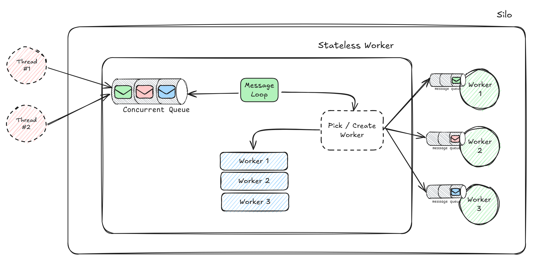
Requests arrive at the SW, and that delegates the actual processing to one of its workers (again, regular grains). A GrainAddress consists of the GrainId, ActivationId, SiloAddress, also MembershipVersion but that is not important right now. The GrainId is the type and the key you specify when you call GrainFactory.GetGrain<IMyGrain>("my-key"). The ActivationId is more, shall we say "neglected" topic, but it really is just a glorified Guid.
The part I want to discuss is the SiloAddress. This address is very important (among other things) to the catalog, and the directory for the grain to be addresable of course. In the context of the SW, in order for the SW to delegate requests to its workers (which are internally referenced by it) they all have to live in the same silo, indicated by the SiloAddress of the GrainAddress to begin with.
This would typically be the silo from where the original call came from, or the target silo if that call came from an external client. There are cases when another silo becomes the host, such as when that specific grain type is incompatible with the silo that received the call for activating the SW. Regardless if its "this" or "that" silo, all workers will be local to the silo which hosts the SW. The differentiating factor between the workers, is the ActivationId.
While the workers are regular grains, they are NOT individually addressable (this is where SW deviates from the virtual actor model). The reason is that the SW needs direct access to their queue, in order to know to which one of them to delegate any incoming request. Techically it is possible to make the workers individually addressable (from outside), but that would require breaking the SW abstraction, and may be unjustified.
Scaling Strategy
Orleans’ SW grains are adept at handling sudden spikes by spawning new activations up to a configurable maximum, or as many as there are available cores.
This scale-up follows these rules:
- Reuse idle workers whenever possible.
- Create new workers only when necessary (up to a predefined limit).
- Prioritize workers with the least waiting count (when all are busy, and limit is reached).
This is really powerful especially when a burst of load is ushered. The downside is that once the burst subsides, these extra activations remain alive until the activation collector reclaims them after a preset period (default 15 minutes).
This delay in scaling down is unneccessary and results in more resource utilization, as idle workers continue consuming memory even when they are no longer needed. Add to it in-memory state, and potentially running timers, and one can see that this is suboptimal.
To overcome this restriction, the solution introduces a dynamic control mechanism that continuously monitors the workers' load, and scales-down the number of workers accordingly, without affecting the existing scale-up strategy.
Adaptive Scale-down
At its core, a PID controller is used to gauge the difference between the current state and the desired state. The current state in our context is the average number of waiting messages (the waiting count) across all of the queues of the workers, and the desired state is zero waiting count.
When the controller detects that the workload has dropped, it emits a control signal which we will use to proactively remove surplus workers.
The overall control function is given by:
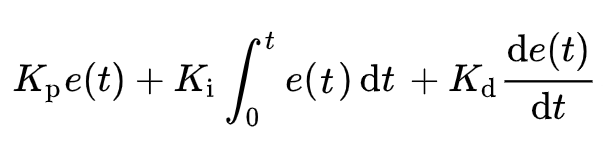
Where e(t) is the most recent error, and Kp, Ki, Kd, are non-negative fixed values, and denote the coefficients for the proportional, integral, and derivative terms respectively.
- Proportional Term - Reacts to the current error between the measured queue length and the desired level. A larger error yields a stronger response.
- Integral Term - Accumulates past errors to eliminate residual biases. This term ensures that the system does not settle with a persistent offset.
- Derivative Term - Predicts the future error based on its rate of change, adding a damping effect that prevents overshooting during rapid fluctuations.
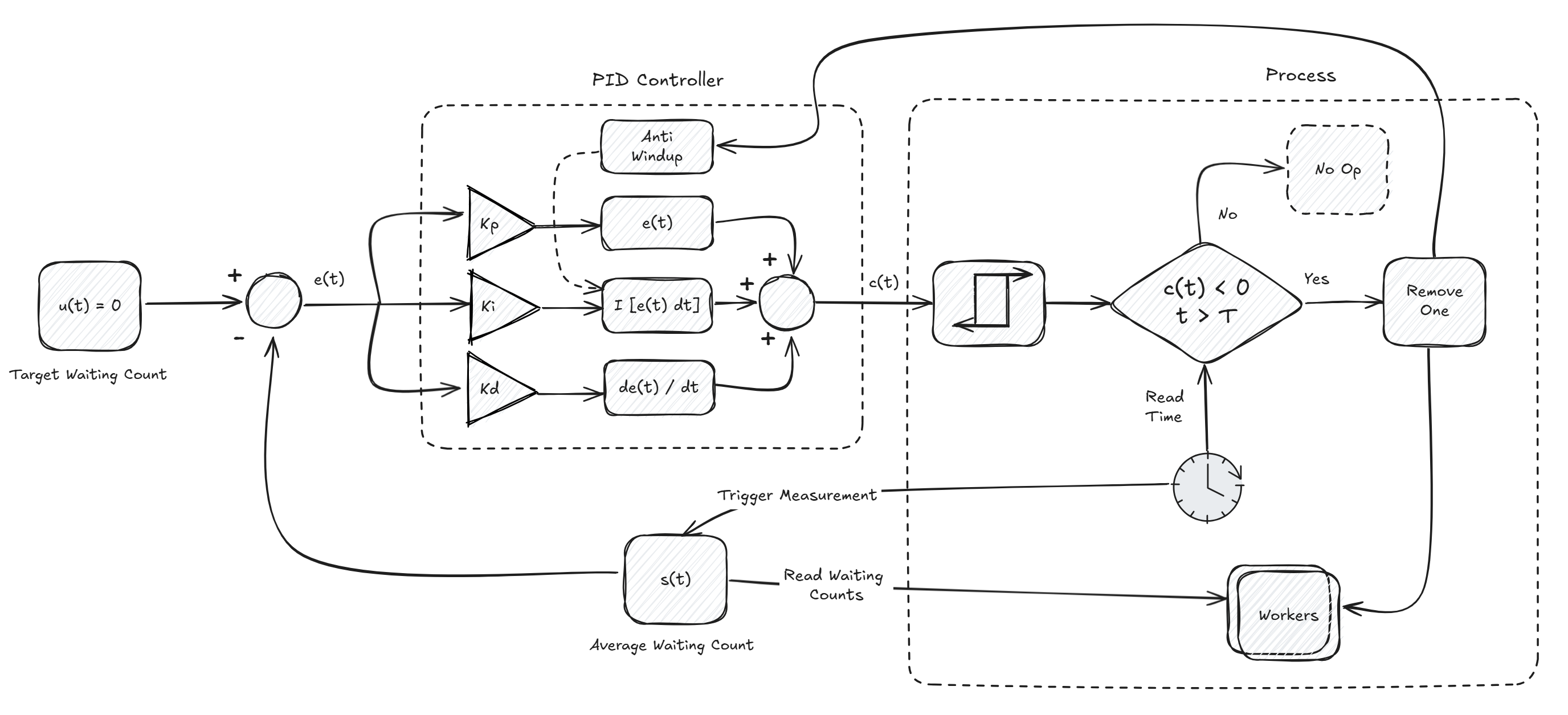
I decided to incoorporate anti-windup too, as it helps prevent the build-up of the integral term, therefor avoiding excessive corrections once constraints are lifted. Such a constraint lifting is achived when we remove a worker.
In addition, I have added a non-ideal hysteresis which introduces a deliberate deadzone which requires a "significant" change to the control signal c(t) before adjusting the control output.
We could have also removed the input signal u(t) as that is always 0, because the target is no waiting count, and the measurement/sensor signal s(t) could just be multiplied by -1. But I have left it in the diagram, so it feels more natural for readers who are familiar with control theory diagrams.
The above can be turned into the following pseudo-code:
timesBelowZeroCount = 0

while true do
   avgWC = ComputeAverageWaitingCount(workers)
   error = -avgWC
   integralTerm = integralTerm + error
   derivativeTerm = error - previousError
   previousError = error
   controlSignal = (Kp * error) + (Ki * integralTerm) + (Kd * derivativeTerm)

   if TimeSince(lastWorkerRemovalTime) > Backoff then
       if controlSignal < 0 then
           timesBelowZeroCount++
           if timesBelowZeroCount > Threshold then
               inactiveWorkers = GetInactiveWorkers()
               if Count(inactiveWorkers) > 0 then
                   worker = SelectRandomWorker(inactiveWorkers)
                   Remove(worker)
                   integralTerm = AntiWindup(integralTerm, inactiveWorkers)
                   lastWorkerRemovalTime = Now
               end if
               timesBelowZeroCount = 0
           end if
       else
           timesBelowZeroCount = 0
       end if
   end if
end while
Parameter Tuning
Finding the parameter values for Kp, Ki, and Kd for the SW removal process is very challenging due to irregular message arrivals and dynamic workload variations. Traditional methods like Ziegler-Nichols assume linearity, but real-world systems are mostly non-linear as they exhibit delays, bursts, and non-stationary behavior, making a data-driven approach more suitable.
In the world of evolutionary algorithms, Gradient-based methods such as the famous gradient descent is very appealing, but in its pure form it suffers from multiple locality problems (minima, maxima, saddle-points). And while there are ways around it, such as simulated annealing, we can get by easier.
I have decided to use a Genetic Algorithm (GA), specifically the real-valued one, to iteratively evolve optimal values. GA operates by maintaining a population of candidate solutions, selecting the best-performing ones, combining their traits through crossover, and introducing mutations to explore new possibilities which lead to a robust tuning mechanism, for a non-linear environment.
The above can be turned into the following pseudo-code:
populationSize ← 20
generations ← 50
mutationRate ← 0.1
population ← []

For i = 1 to populationSize:
    Kp ← Abs(Random(0, 1))
    Ki ← Abs(Random(0, 1))
    Kd ← Abs(Random(0, 1))
    population ← (Kp, Ki, Kd)

For generation = 1 to generations do:
   Compute fitness for each individual:
     fitness ← []
     For each (Kp, Ki, Kd) in population:
         score ← CalculateFitnessScore(Kp, Ki, Kd, messageArrivalTimes)
         fitness ← (Kp, Ki, Kd, score)

   Select individuals based on lowest fitness score:
      Sort fitness by score in ascending order
      bestIndividuals ← First(populationSize / 2)

   Generate new population:
     newPopulation ← []
     While size(newPopulation) < populationSize:
         parent1 ← Random(bestIndividuals)
         parent2 ← Random(bestIndividuals)
         childKp ← Abs((parent1.Kp + parent2.Kp) / 2)
         childKi ← Abs((parent1.Ki + parent2.Ki) / 2)
         childKd ← Abs((parent1.Kd + parent2.Kd) / 2)

         If Random(0,1) < mutationRate:
             childKp ← Abs(childKp + Random(-0.05, 0.05))
             childKi ← Abs(childKi + Random(-0.05, 0.05))
             childKd ← Abs(childKd + Random(-0.05, 0.05))

         newPopulation ← (childKp, childKi, childKd)

   Replace population with newPopulation

Compute fitness for final population:
  fitnessValues ← []
  For each (Kp, Ki, Kd) in population:
      score ← CalculateFitnessScore(Kp, Ki, Kd, messageArrivalTimes)
      fitnessValues ← (Kp, Ki, Kd, score)

Find best individuals:
  bestFitness ← Min(fitnessValues)
  bestSolutions ← All(Kp, Ki, Kd) where Abs(score - bestFitness) < Tolerance

If bestSolutions is empty
  return [(1.2, 0.4, 0.3)] // some defaults
Else
  return bestSolutions
Fitness Score
The above pseudo-code describes the GA itself, and you may have noticed that part of the algorithm is the calculation of the fitness score. The fitness score is a real-value (guess where the name comes from) representing how well a given set of PID parameters performs in controlling the SW removal process.
The idea is to build a simulation of the SW removal process, which takes any given PID parameters, and some way of generating message arrival patterns. We than continuously measure some key metrics, and compute the fitness score from those metrics. The lower the fitness score, the better the parameter values.
The above can be turned into the following pseudo-code:
  Kp ← Random(0, 1)
  Ki ← Random(0, 1)
  Kd ← Random(0, 1)

RunSimulation(Kp, Ki, Kd)

While simulationRunning:
  queueLength ← ComputeQueueLength()
  waitingTime ← ComputeWaitingTime()
  overshoot ← ComputeOvershoot()
  settlingTime ← ComputeSettlingTime()
  fitnessScore ← CalculateFitnessScore(queueLength, waitingTime, overshoot, settlingTime)

Evolve (Kp, Ki, Kd) using GA:
  For generation = 1 to maxGenerations do:
    Select best-performing individuals
    Apply crossover to produce new candidates
    Apply mutation with probability mutationRate
    Evaluate new candidates and update population

Return (Kp, Ki, Kd) ← Lowest(fitnessScore)
The core is to generate very different message arrival patterns, so that that GA has a variable pool to work with, and after each simulation the best PID values are stored, and in the end they are averaged out to find a single value, for each of the parameters.
Below we can see a series of simulations, with different arrival patterns, but all sharing the same final PID values. On each one of them, we present 4 graphs, that all have the same x-axis (time). On the y-axis we have the following quantities:
- Message Rate - The rate of incoming messages that hit the SW.
- Worker Count - The total number of workers the SW has.
- Queue Length - The total number of pending messages on the SW itself.
- Avg Waiting Count - The average number of pending messages across all the worker's queue.
- Blue-colored plots show the current behavior in Orleans, also labeled as static in the legend.
- Red-colored plots show the new behavior in the simulations, also labeled as dynamic in the legend.
- The dotted plots show the average value across the simulation of their solid counterparts.
Constant Pattern
A fixed rate produces equally spaced messages. The tiny fluctuations are because of rounding errors.
Static: Avg Workers = 30.815, Avg Queue Length = 0.25333333333333335
Dynamic: Avg Workers = 29.655, Avg Queue Length = 0.31666666666666665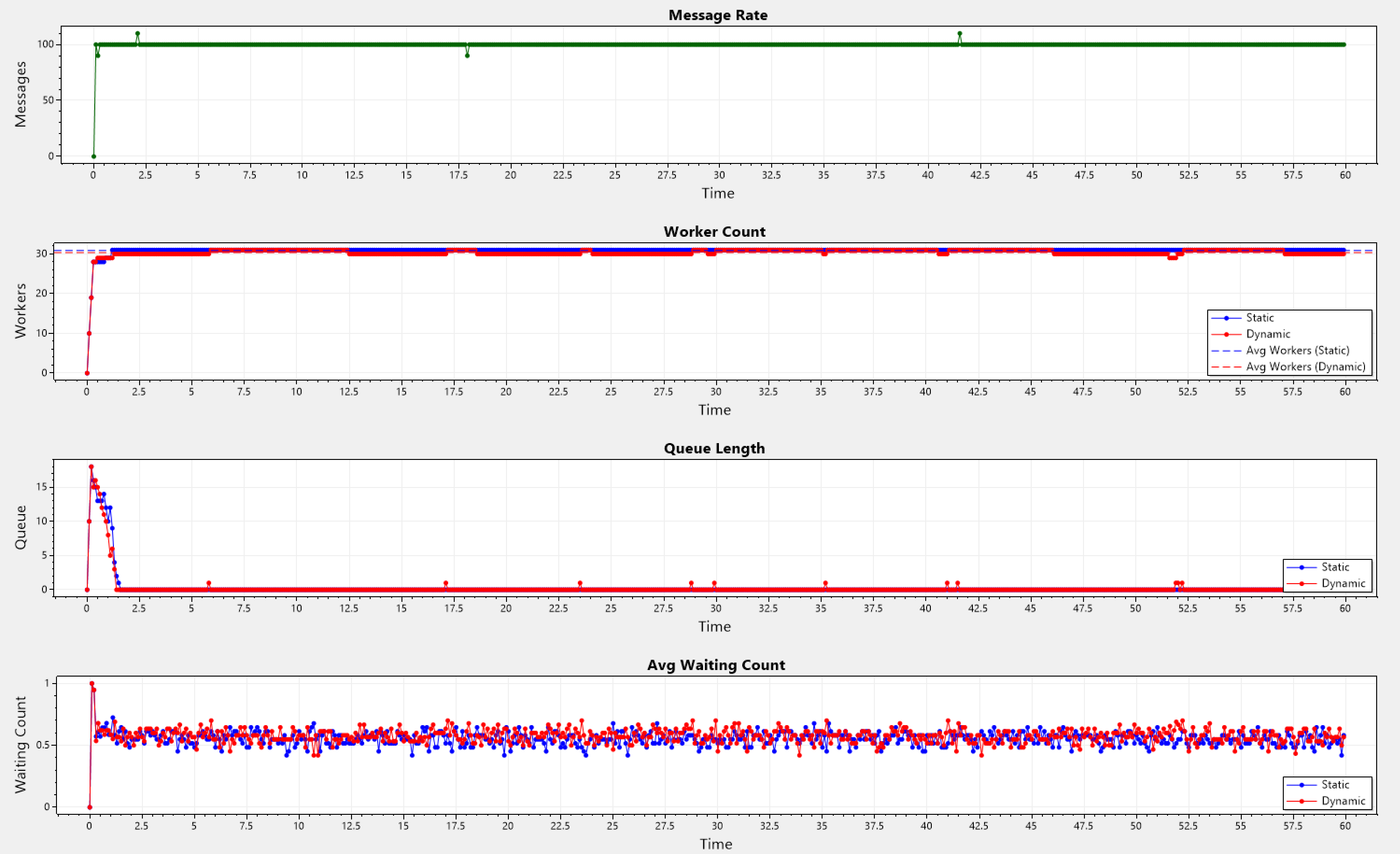
Periodic Pattern
A base-rate is used which gets reduced during designated low‐rate periods. Also, a small random noise of ±0.5 is added to the rate factor.
Static: Avg Workers = 29.265, Avg Queue Length = 0.23166666666666666
Dynamic: Avg Workers = 28.393333333333334, Avg Queue Length = 0.36666666666666664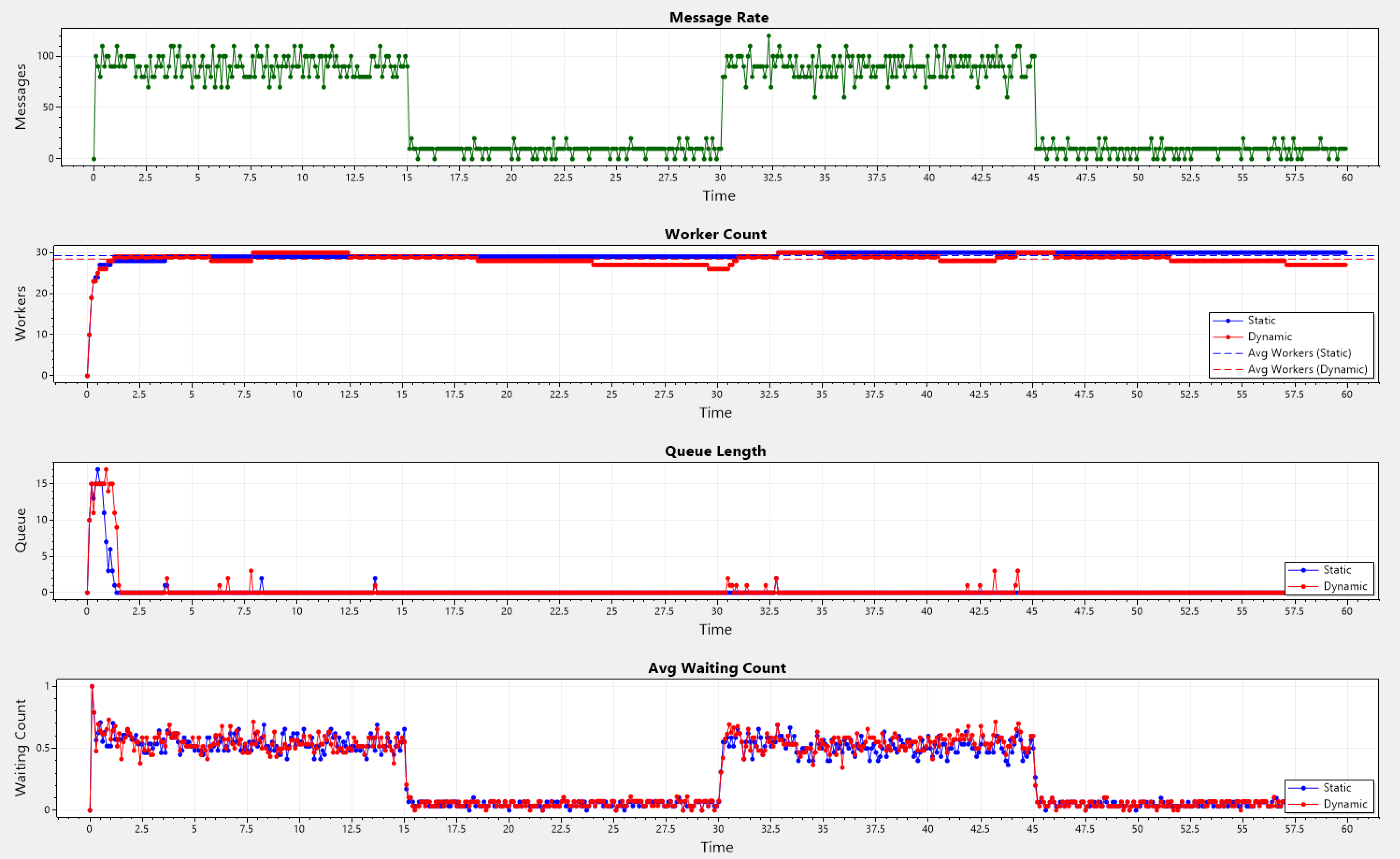
Ramp Pattern
The rate increases linearly (ramp-up) until the midpoint of the simulation, then decreases linearly (ramp-down). Bounded randomness is introduced at each point.
Static: Avg Workers = 22.13, Avg Queue Length = 0.10333333333333333
Dynamic: Avg Workers = 20.268333333333334, Avg Queue Length = 0.08666666666666667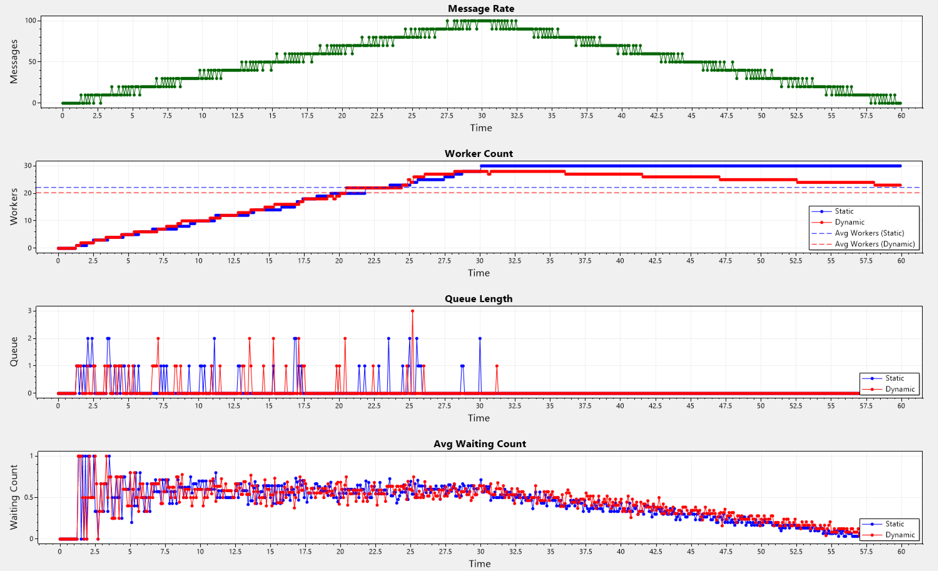
Spike Pattern
At fixed intervals, a spike occurs over a short duration during which a number of messages are generated.
Static: Avg Workers = 4.1583333333333334, Avg Queue Length = 0.075
Dynamic: Avg Workers = 3.66, Avg Queue Length = 0.07166666666666667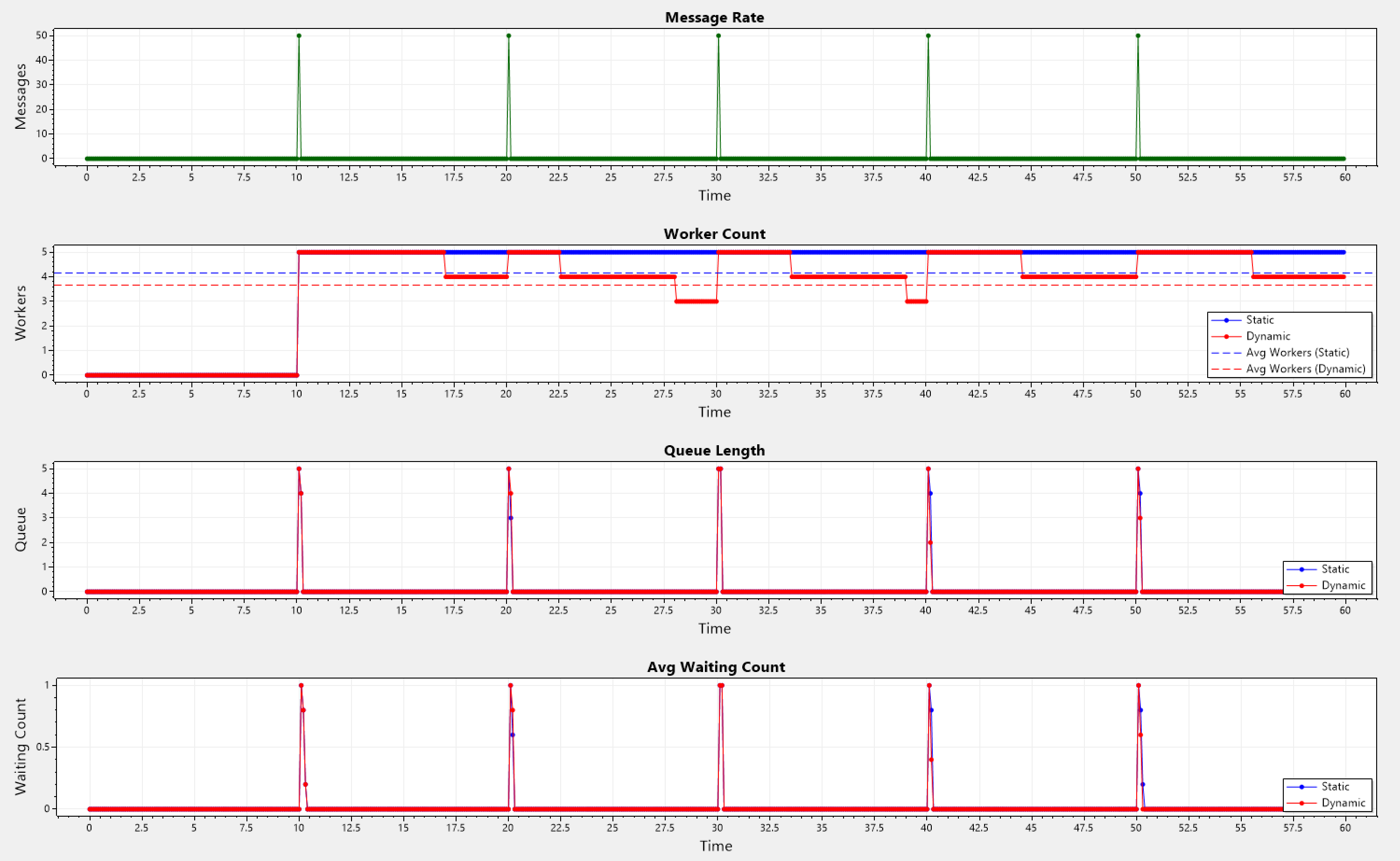
Burst Pattern
A sudden spike in the arrival rate is introduced, followed by a steady-state rate, which than is followed by an exponential decay back to a zero rate. Spikes happen at a-periodic intervals.
It may look a bit counter-intuitive on why the dynamic plot shows almost the same number of workers, consistently! That is because of the high number of messages at each spike ~500, and the limited number of workers. Note that processing time is accounted for, in each simulation.
Static: Avg Workers = 49.915, Avg Queue Length = 49.373333333333335
Dynamic: Avg Workers = 49.045, Avg Queue Length = 49.20333333333333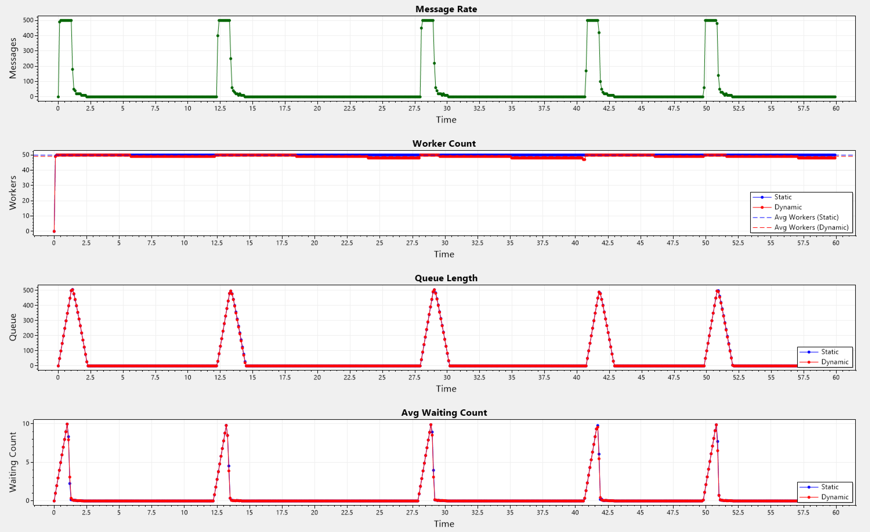
Chaotic Pattern
This pattern uses a low base-rate most of the time, but with a chance of triggering a spike with a higher, yet randomly determined rate.
Static: Avg Workers = 20.328333333333333, Avg Queue Length = 0.2916666666666667
Dynamic: Avg Workers = 16.971666666666668, Avg Queue Length = 0.31666666666666665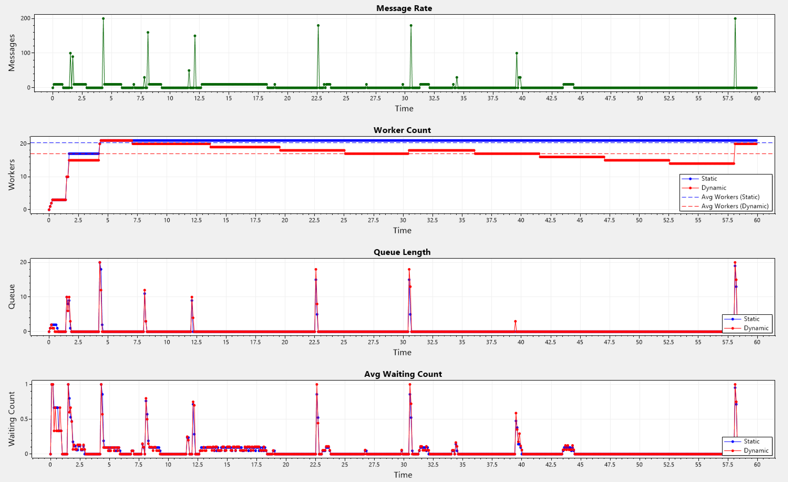
It is somewhat expected that running the simulations with the final PID values, would yield good results on the metrics. This is beacause those parameters were tuned on the same metrics that resulted from the same arrival patterns. The real test is to see how the simulation performs (with the same PID values), but for a wildly different pattern.
Poisson Pattern
In a Poisson distribution, the probability of an event occurring in the next instant, does not depend on when the last event happened. This means arrivals are purely random, unlike the other patterns with semi-fixed intervals or feedback mechanisms.
Therefor a Poisson arrival pattern would be fundamentally different from the other patterns, because it models independent, and memory-less message arrivals. Many systems including internet traffic exhibit Poisson-like behavior, making it a fitting benchmark.
Static: Avg Workers = 42.358333333333334, Avg Queue Length = 0.37666666666666665
Dynamic: Avg Workers = 38.615, Avg Queue Length = 0.43166666666666664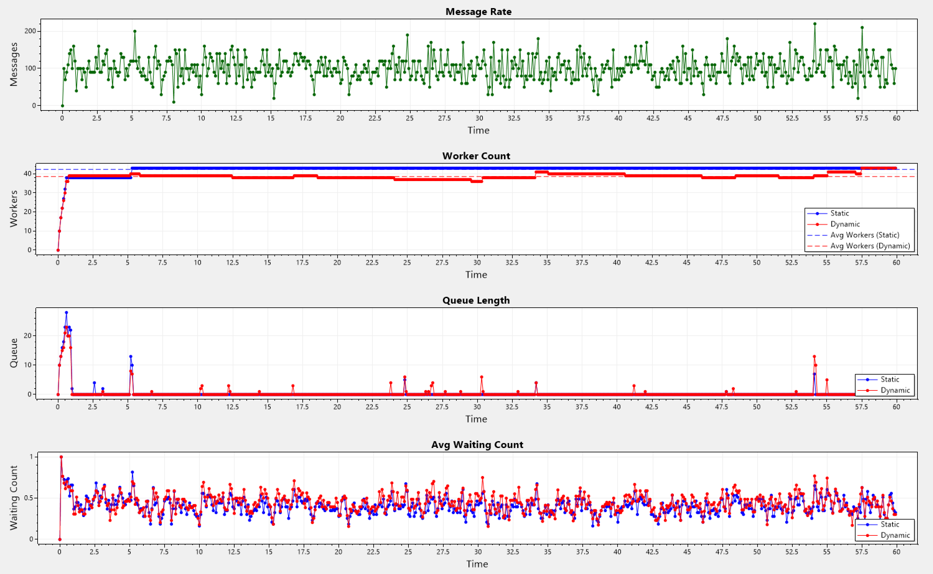
All of the simulations showcase very close average number of workers, because they are designed in such a way that they stress-test the approach under conditions of perpetual activity. Otherwise when activity cools down, the effect would be way more apparent.
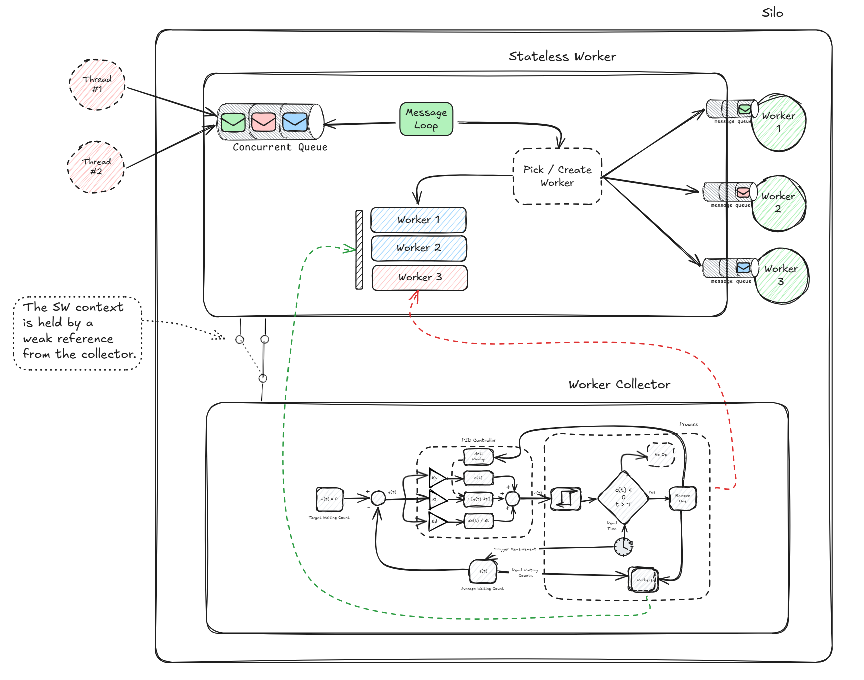
Implemention Detail
I have implemented this idea in Orleans, and the below diagram is a good representation of the real thing. Pretty much all we talked above is part of it, one thing I would like to note here is this weird looking connection between the SW context and the worker collector.
The idea was that this would complement the SW, and that only when requested by the developer, and not a thing that is "on" by default. The implementation requires extra fields within the context, and of course has a tiny overhead, for that reason I did not want that overhead when its not used.
Therefor the collector (the implementation of what we talked thus far) is an external component that can be hooked into the SW context. The connection is made via a weak reference, so that the collector remains alive as long as the associated context is, without unintentionally extending its lifetime and preventing it (SW context) from being collected by the .NET GC.
This is important to avoid memory leaks, as a SW context is NOT subject to the grain activation collector.
There is zero overhead if you do not decided to make use of it.
Benchmark Results
The benchmark can be summarized as follows:
- Setup - The benchmark tests the performance of two types of SW grains (monotonic & adaptive), using a Poisson process for arrival rates.
- Metrics - Collects and reports worker metrics, including active, maximum, and average workers, over the benchmark duration.
- Evaluation - After each execution, multiple cooldown cycles are applied based on the benchmark configuration. During this time, metrics collection continues.
The cooldown period is a round up of 1/10th the process delay and the ratio of concurrent tasks to the maximum worker limit. The average worker statistics on each run, is rounded via banker's rounding midpoint scheme. This is repeated over 10 iterations.
Monotonic Grain Results
Active and average worker counts remain constant during each cooldown cycle, showcasing the lack of adaptive scale-down.
Executing benchmark for SWMontonicGrain

Waiting for cooldown (1/10)

Stats (1/10):
 Active Workers:  10
 Average Workers: 10
 Maximum Workers: 10

-------------------------------------------

Waiting for cooldown (2/10)

Stats (2/10):
 Active Workers:  10
 Average Workers: 10
 Maximum Workers: 10

-------------------------------------------

Waiting for cooldown (3/10)

Stats (3/10):
 Active Workers:  10
 Average Workers: 10
 Maximum Workers: 10

-------------------------------------------

Waiting for cooldown (4/10)

Stats (4/10):
 Active Workers:  10
 Average Workers: 10
 Maximum Workers: 10

-------------------------------------------

Waiting for cooldown (5/10)

Stats (5/10):
 Active Workers:  10
 Average Workers: 10
 Maximum Workers: 10

-------------------------------------------

Waiting for cooldown (6/10)

Stats (6/10):
 Active Workers:  10
 Average Workers: 10
 Maximum Workers: 10

-------------------------------------------

Waiting for cooldown (7/10)

Stats (7/10):
 Active Workers:  10
 Average Workers: 10
 Maximum Workers: 10

-------------------------------------------

Waiting for cooldown (8/10)

Stats (8/10):
 Active Workers:  10
 Average Workers: 10
 Maximum Workers: 10

-------------------------------------------

Waiting for cooldown (9/10)

Stats (9/10):
 Active Workers:  10
 Average Workers: 10
 Maximum Workers: 10

-------------------------------------------

Waiting for cooldown (10/10)

Stats (10/10):
 Active Workers:  10
 Average Workers: 10
 Maximum Workers: 10
 -------------------------------------------
Adaptive Grain Results
Active and average worker counts decrease over each cooldown cycle, showcasing the presence of adaptive scale-down.
Executing benchmark for SWAdaptiveGrain

Waiting for cooldown (1/10)

Stats (1/10):
 Active Workers:  8
 Average Workers: 9
 Maximum Workers: 10

---------------------------------------------------------------------

Waiting for cooldown (2/10)

Stats (2/10):
 Active Workers:  7
 Average Workers: 9
 Maximum Workers: 10

---------------------------------------------------------------------

Waiting for cooldown (3/10)

Stats (3/10):
 Active Workers:  6
 Average Workers: 9
 Maximum Workers: 10

---------------------------------------------------------------------

Waiting for cooldown (4/10)

Stats (4/10):
 Active Workers:  5
 Average Workers: 9
 Maximum Workers: 10

---------------------------------------------------------------------

Waiting for cooldown (5/10)

Stats (5/10):
 Active Workers:  4
 Average Workers: 8
 Maximum Workers: 10

---------------------------------------------------------------------

Waiting for cooldown (6/10)

Stats (6/10):
 Active Workers:  3
 Average Workers: 8
 Maximum Workers: 10

---------------------------------------------------------------------

Waiting for cooldown (7/10)

Stats (7/10):
 Active Workers:  2
 Average Workers: 8
 Maximum Workers: 10

---------------------------------------------------------------------

Waiting for cooldown (8/10)

Stats (8/10):
 Active Workers:  2
 Average Workers: 8
 Maximum Workers: 10

---------------------------------------------------------------------

Waiting for cooldown (9/10)

Stats (9/10):
 Active Workers:  1
 Average Workers: 7
 Maximum Workers: 10

---------------------------------------------------------------------

Waiting for cooldown (10/10)

Stats (10/10):
 Active Workers:  0
 Average Workers: 7
 Maximum Workers: 10

---------------------------------------------------------------------
If you found this article helpful please give it a share in your favorite forums 😉.
The solution project for the simulations is available on GitHub.