

Introduction
In a previous article I have gone in-depth about the theory behind Memory-aware rebalancing (MAR), and a good technical explaination can be found here. I have briefly mentioned Locality-aware rebalancing (LAR), but a good technical explaination on LAR can be found here, while a theoretical one can be found here.
LAR and MAR are two mechanisms that govern grain activation rebalancing, and cutting cross-communications between activations.
LAR dynamically adjusts activation placement to respect communication locality. It runs continuously, and is constrained to avoid de-balancing an already balanced cluster.
MAR reacts to cluster imbalances by means of redistributing activations. It runs periodically, or on-demand, and is constrained on the number of activations to relocate, but only within a rebalancing cycle.
Mind you that both LAR and MAR are designed to operate independently, so neither makes assumptions about the other. It can become a problem though when they are used simultaneously.
- MAR can temporarily disrupt LAR's locality corrections.
- LAR can interfere with MAR's rebalancing corrections.
We can overcome those challenges, because MAR enables developer control, and while LAR does not, it does expose the IImbalanceToleranceRule, which represents a rule that controls the degree of imbalance between the number of grain activations (that is considered tolerable), when any pair of silos are exchanging activations between them.
Cluster Imbalance & Tolerance Rule
MAR exposes a cluster-wide rebalancing report, either on-demand by requesting it via the IActivationRebalancer, or you can subscribe and listen to report updates.
I will not go into the details of the parameters and options, since they are not relevant here, but the report has a property called ClusterImbalance.
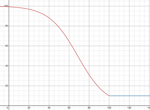
Orleans, comes with a default implemention for IImbalanceToleranceRule. The rule follows a piecewise, inverted, scaled and shifted, sigmoid function which maps the number of active silos to different tolerance levels.
Below we can see a graph on how this changes, where the x-axis represents the number of silos, and the y-axis is the percentage deviation from the baseline value (set to 10).
The interface is really simple:
public interface IImbalanceToleranceRule
{
    bool IsSatisfiedBy(uint imbalance);
}
IsSatisfiedBy accepts a parameter called imbalance. This has nothing to do with MAR's reported ClusterImbalance, the repartitioner is the one that supplies that value, but in the current implementation, that value represents the imbalance that will result in, between the exchanging silos, if this method were to return true.
In other words, the default rule, and the repartitioner, have no knowledge about the cluster's imbalance.
A strategy to allow for the coexistence LAR-MAR, is for the tolerance rule to account for the cluster imbalance. And given that we can get the cluster imbalance, we can influence LAR to be less tolerant when imbalance is high, and the opposite (or rather bounce back to baseline) when imbalance is low.
Nothing stops the developer from defining their own tolerance rule, it just needs to be aware and scale accordingly to the cluster's imbalance.
It is clear that there must exist some kind of tolerance conversion factor, that ties these together, the question is which one is it?
Conversion Factor Derivation
Throughout the article I mention that m > 0, yet I define boundary conditions such as f(0) and g(0). This can sound contradictory, but we can define a function f(x) for x > 0, and yet impose a boundary condition at x = 0, especially in the context of differential equations, where boundary conditions are often specified at the endpoints of a domain. We can resort to the limit of f(x) as x → 0+ (from the right side), so long as the boundary condition is compatible with that limit.
We will postulate that whatever the factor is, it must be:
- A continuous function
f, as the cluster imbalancemis a fluctuating, double precision, floating point number. - Depended on the cluster imbalance, so
f(m). - Bounded in the (0, 1) range, in order to achive normalization.
Given the posulates above, we can formulate the following conditions.
Boundary Conditions
- When
m = 0, the cluster is perfectly balanced, so we want maximum tolerancef(0) = 1. - When
m = 1, the cluster is fully imbalanced, so we want no tolerancef(1) = 0.
This anchors the function at both ends and gives it well-defined start and end values.
Monotonicity
f'(m) < 0, m ∈ (0, 1)
f(m) is strictly monotonically decreasing, because its first derivative (the slope) is constantly negative. In other words, as imbalance increases, tolerance must decrease.
Concavity
f"(m) < 0, m ∈ (0, 1)
The rate of decrease itself increases i.e. the curve is concave down (or simply 'concave'). In other words, the drop in tolerance accelerates as imbalance grows. This would have to be manifested as:
- For
m ~ 0; Weakest suppression, LAR can optimize for locality. - For
m ~ 1; Strongest suppression, MAR can optimize for imbalance.
To satisfy these conditions, and knowing that we do not have (yet) a general form for f(m), we begin with its first derivative and model it as: f'(m) = -k⋅g(m), where f(m) is the tolerance conversion factor (or rather curve), and g(m) is the shape of the rate at which f falls.
Since we expressed f'(m) in terms of g(m) and the proportionality constant -k, in order for the monotonicity condition of f to hold, it must than by extension follow that g(m) > 0, m ∈ (0, 1).
Much the same way as with f(m) we state the boundary conditions for g(m) (which are the opposites)
- When
m = 0, the cluster is perfectly balanced, so we want the rate at which tolerance falls to be zero, thereforg(0) = 0. - When
m = 1, the cluster is fully imbalanced, so we want the rate at which tolerance drops to be at its highest, thereforg(1) = 1.
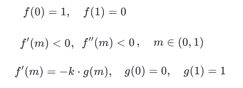
The boundary, monotonicity, and concavity conditions for f(m) and g(m) are expressed below.
We first integrate f'(m) without specifying limits. This gives us the indefinite integral, where C is the constant of integration. Using the fundamental theorem of calculus, we can reinterpret the indefinite integral, to a definite one on the range (0, m). Then, using the boundary condition f(0) = 1, we can come to a general form for f(m).
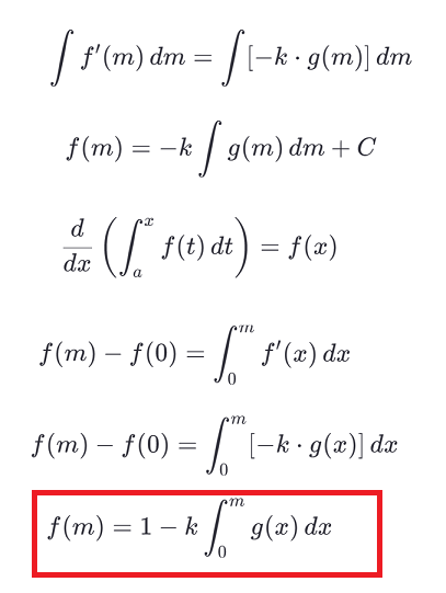
We will make use of the highlighted equation later on.
Given the concavity condition f"(m) < 0, m ∈ (0, 1), and the general form of the first derivative f'(m) = -k⋅g(m), it follows that f"(m) = -k⋅g'(m) < 0. In order for this to hold true, it must mean that g'(m) > 0, thus g(m) must be strictly increasing.
We want the rate of tolerance reduction to accelerate with m, therefor we impose an additional constraint. Knowing that m ∈ (0, 1), it means that m > 0, which also means m2 > 0. This allows us to multiply by m2, and divide by m, without having to change the inequality direction, and using the quotient rule for derivatives, we get the following.
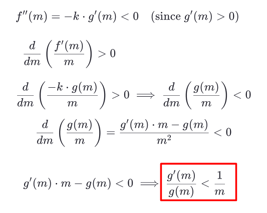
The highlighted equation shows that the relative growth rate: g'(m)/g(m) is less than 1/m, which tells us that g(m) grows sublinearly with respect to m.
A function is said to grow sublinearly with respect to some variable, if its growth rate slows down as the variable increases. Mathematically, this means that the derivative of it decreases over the (increasing) variable, and that the ratio between it and the variable, becomes smaller as the variable increases.
This key insight allows us to make an educated guess around the nature of g(m), and given the boundary conditions of g(m), we get the following.
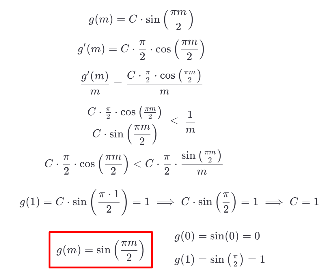
The highlighted equation shows that g(m) = sin(πm/2), statisfies all boundary conditions, monotonicity, concavity, and the sublinear growth. It is the right rate at which the tolerance conversion factor should fall. This tells us that f(m) follows a small decrease when m is small (which means low imbalance), and starts ramping up as m → 1 (full imbalance), then reverses in the opposite order as m → 0 (zero imbalance).
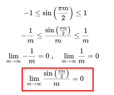
We can prove that g(m) = sin(πm/2) is sublinear, because the limit of g(m) divided by m, as m → ∞, is zero. Because g(m) is a bounded oscillatory function, it means that -1 <= sin(πm/2) <= 1, regardless of the value of m. Since m > 0 we can divide both sides with m without having to change the inequality direction. Also, knowing that the limits of 1/m and -1/m, as m → ∞, are both zero, we can apply the squeeze theorem, and thereby prove that the limit of g(m) must also be zero.
Below we can see five graphs. Do not get to caught up with the fact that some of the functions, are above the g(m) = m line, it is the trend of growth that defines it.
- Black →
g(m) = m| A function which grows linearly. - Orange →
g(m) = ln(m)| A function (below the x-axis) which grows sublinearly, but fails to statisfy the boundary conditions. - Violet →
g(m) = sin(m)| A function which grows sublinearly, but fails to statisfy the boundary conditions. - Red →
g(m) = sqrt(m)| A function which grows sublinearly, statisfies the boundary conditions, but fails on the concavity condition. - Blue →
g(m) = sin(πm/2)| A function which grows sublinearly, and statisfies all imposed conditions.
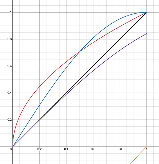
We can see that g(m) = sqrt(m) would have also worked, but there is a subtle difference. Note how it exibits the opposite of sin(πm/2) i.e. when m ~ 0 is starts more aggressive, which translates to a faster fall of f(m), the interpretation is that the tolerance factor would react more quickly on low cluster imbalance, and slow down as imbalance becomes larger m ~ 1.
This is against the concavity condition, and not the desired behavior. We want it to be more aggressive when imbalance is trending towards 1. Interestingly enough, if we would have used 1/m as the metric, i.e. the cluster's balance (as opposed to imbalance), than it would have worked out.
Given this information, and the general form of f(m) that we derived earlier, we can perform a u-substitution for: g(x)⋅dx over (0, m), and knowing the boundary condition f(1) = 0, we can find the proportionallity constant to be k = π/2. Than we arrive to the final form of f(m) = cos(πm/2), which is the tolerance conversion factor.
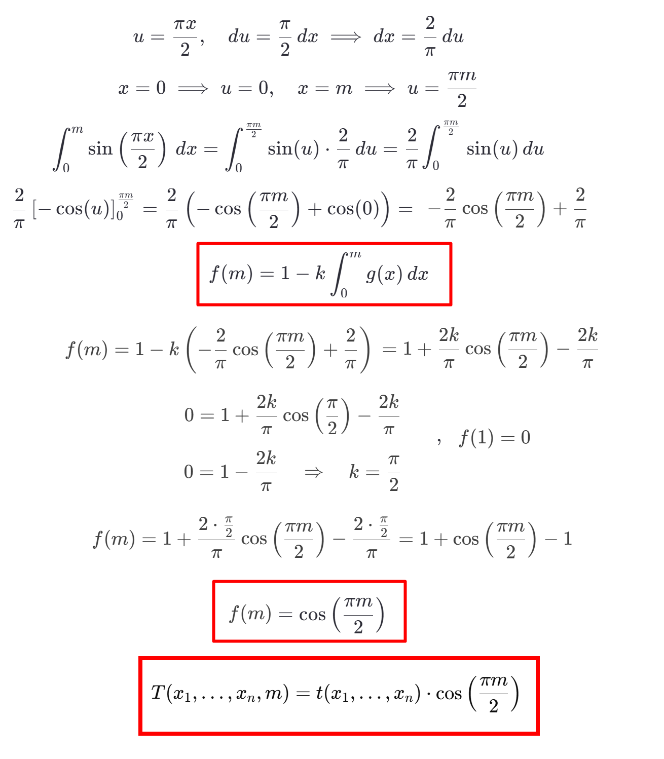
There are 3 highlighted equations, the first one is the general form of f(m) that we derived earlier, the second is the tolerance conversion factor (what we were after for), and the third one T(x1,...xn, m), is a multi-variable, cluster-aware tolerance rule, which has some t(x1,...xn) implementation, multiplied by the conversion factor to allow for LAR-MAR coexistence. t(x1,...xn) can be any rule i.e. the current silo-aware one in Orleans, a more complicated one that takes other factors into consideration, or something as simple as a static threshold value.
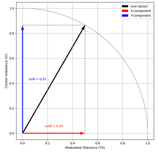
Geometric Interpretation
The unit circle provides an nice visualization for the tolerance-imbalance conservation. At an angle θ = πm/2, the unit vector components are:
- Red →
cosθ| The modulated toleranceT/t - Blue →
sinθ| The imbalance penalty
Balanced State (θ = 0):
- The unit vector lies along the x-axis → Full tolerance (
cos0 = 1) - The y-component is 0 → No imbalance (
sin0 = 0)
Imbalanced State (θ = π/2):
- The unit vector points lies along the y-axis → Zero tolerance (
cos(π/2) = 0) - The y-component is 1 → Full imbalance (
sin(π/2) = 1)
The pythagorean trigonometric identity cos²θ + sin²θ = 1 enforces strict conservation - an increasing imbalance necessarily requires reduction of the tolerance. This geometric approach enforces the idea of the tolerance factor f(m) = cos(πm/2) that automatically scales LAR's corrections based on MAR's imbalance metric.
The moduled tolerance can be seen as a projection of the unit vector (which conserves the relationship) onto the x-axis. Overall this guarantees proper coupling between LAR and MAR without requiring manual tuning.
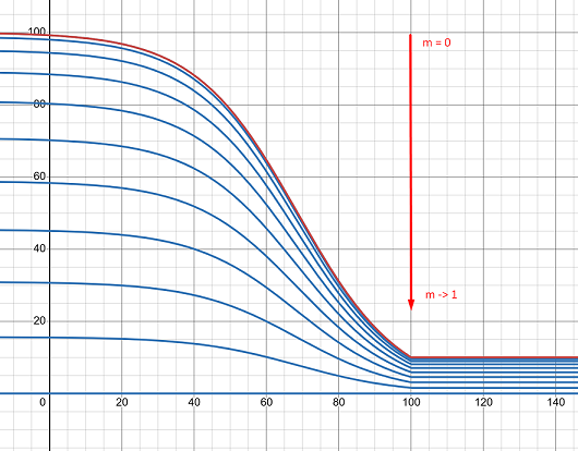
Rebalancer-compatible Rule
Below we can see one red, and a series of blue graphs. The red graph shows how the default pairwise imbalance tolerance rule scales with the number of silos (essentially the graph we showed at the begining), while the blues once represent a new tolerance rule which scales not only with the number of silos, but also with the cluster's imbalance. The tolerance factor is taken into consideration, and the blue graphs themselves are Δm = 0.1 apart.
Below I have provided the implementation of such a rule. This is just an example, your rule can be totally different, yet the conversion factor would stay valid.
public class RebalancerCompatibleRule(IServiceProvider provider) :
    IImbalanceToleranceRule, ILifecycleParticipant<ISiloLifecycle>,
    ILifecycleObserver, ISiloStatusListener, IActivationRebalancerReportListener
{
    private readonly object _lock = new();
    private readonly Dictionary<SiloAddress, SiloStatus> _silos = [];

    private uint _pairwiseImbalance;
    private double _clusterImbalance;

    private readonly ISiloStatusOracle _oracle = provider.GetRequiredService<ISiloStatusOracle>();
    private readonly IActivationRebalancer? _rebalancer = provider.GetService<IActivationRebalancer>();

    public bool IsSatisfiedBy(uint imbalance) => imbalance <= Volatile.Read(ref _pairwiseImbalance);

    public void SiloStatusChangeNotification(SiloAddress silo, SiloStatus status)
    {
        lock (_lock)
        {
            ref var statusRef = ref CollectionsMarshal.GetValueRefOrAddDefault(_silos, silo, out _);
            statusRef = status;
            UpdatePairwiseImbalance();
        }
    }

    public void Participate(ISiloLifecycle lifecycle)
        => lifecycle.Subscribe(nameof(RebalancerCompatibleRule),
               ServiceLifecycleStage.ApplicationServices, this);

    public void OnReport(RebalancingReport report)
    {
        lock (_lock)
        {
            _clusterImbalance = report.ClusterImbalance;
            UpdatePairwiseImbalance();
        }
    }

    private void UpdatePairwiseImbalance()
    {
        var activeSilos = _silos.Count(s => s.Value == SiloStatus.Active);
        var percentageOfBaseline = 100d / (1 + Math.Exp(0.07d * activeSilos - 4.8d));

        if (percentageOfBaseline < 10d) percentageOfBaseline = 10d;

        var pairwiseImbalance = (uint)Math.Round(10.1d * percentageOfBaseline, 0);
        var toleranceFactor = Math.Cos(Math.PI * _clusterImbalance / 2);

        _pairwiseImbalance = (uint)Math.Max(pairwiseImbalance * toleranceFactor, 0);
    }

    public Task OnStart(CancellationToken cancellationToken)
    {
        _oracle.SubscribeToSiloStatusEvents(this);
        _rebalancer?.SubscribeToReports(this);

        return Task.CompletedTask;
    }

    public Task OnStop(CancellationToken cancellationToken)
    {
        _oracle.UnSubscribeFromSiloStatusEvents(this);
        _rebalancer?.UnsubscribeFromReports(this);

        return Task.CompletedTask;
    }
}
If you found this article helpful please give it a share in your favorite forums 😉.