

Introduction
Orleans ensures that when a grain call is made there is an instance of that grain available in memory on some server in the cluster to handle the request. This is called "grain placement". There are a set of out-of-the-box placement strategies that developers can make use of, such as:
- Random
- Hash-based
- Prefer local
- Silo-role
- Activation-count
- Stateless-worker
Resource-based Placement (RBP)
For the once in the audience that are not aware, I've recently published a package which performs grain placement in an attempt to achieve approximately even load, based on cluster resources. It assigns weights to silo runtime statistics to prioritize different properties (cpu usage, memory usage, available memory) and calculates a normalized score for each silo. The silo with the lowest score is chosen for placing the activation. Normalization ensures that each property contributes proportionally to the overall score. The users can adjust the weights based on their specific requirements and priorities for load-balancing.
Main Factors
As with any, what I would like to call "sampling-based" placement strategy, there are 3 main factors that play an important role to an efficient grain placement:
- Frequency of Measurements.
- Silo Selection Algorithm.
- Quality of Measurements.
Frequency of Measurements
In any case, high-frequency measurements always lead to a more predictable and efficient grain placement. This is simply natural, as the placement strategy has more information to work with to make an optimal decision. Low-frequency measurements have a higher chance of missing potentially crucial data-points, which could result in forwarding grain activations towards a silo that is already at working capacity, all because of a prior measurement that showed a subsentially lower load on that silo, while an influx of requests came right after that last measurement.
RBP uses a default period of 1 second to collect resource statistics from all the silos in a cluster. As mentioned, using a shorter period (higher frequency) is more beneficial, but we need to take into account, that a faster cycle results in more calls to the membership grain, so its up to the developer to play with picking the "right" period.
Silo Selection Algorithm
As with activation-count placement, RBP internally uses the Power of K-Choices (PowK) load-balancing algorithm for silo selection. The PowK algorithm is used to distribute incoming tasks or requests among K servers (silos in our case), optimizing resource utilization. By considering multiple choices, it enhances system efficiency by dynamically adapting to varying loads and preventing overloading of specific servers, ensuring a balanced distribution of work.
Typically K = 2; which still results in much better work distribution among the silos than say random choice does. To understand this more intuitively, consider the following:
Imagine a scenario with three servers: A, B, and C. If you always randomly choose a server for a new task, there's a higher chance you might consistently pick the busiest server, leading to an uneven workload. With the power of 2-choices, you randomly pick two servers (say A and B), and then you assign the task to the server with the lighter load. This way, even if one server is busy, you have a backup choice. It's literality like having a plan B.
While K = 2 subsequently improves task distribution over a single random choice, it makes natural sense that picking a higher K-value, leads to even better choices being made. As a matter of fact, for K = n; n being the total number of servers in a cluster, PowK becomes the Join the Shortest Queue (JSQ) algorithm, which originates from the field of queueing theory.
It has been proven here & here that JSQ is optimal among policies that do not know job durations, under several optimality criteria. I mention that its optimal when the job duration is not known, which aligns with the grain placement in Orleans as the runtime has no idea how long this grain will stay activated.
JSQ is usually not deployed in practise when the number of servers in a cluster grows really large, due to the added overhead of pull-based server querying. In push-based systems (like Orleans statistics collector) this does not represent a problem, but the selection itself theoretically reaches a point of diminishing returns.
In RBP, I have decided to go with a K-value which is grows with the square root of the number of silos, as it shows (based on simulations) slightly better selection choices when the number of silos grows. It simply feels unnatural to stick with just K = 2, especially when the number of silos grows in the 100s or 1000s in a cluster. I believe we place an unneccessary restriction by fixing this value.
Quality of Measurements
While the frequency of statistics measurements is imporant, so is the quality of the measurements themselves. Let me try to explain what I mean by "quality". If we think about statistics for a resource like CPU usage, one thing that is inevitable are fluctuations. And I am not just talking about random minuscule fluctuations, but also rapid changes in CPU usage, due to actual work being performed by the tasks, or speaking in the context of Orleans the work being done by the activated grains. The resource consumption can be widely inconsistent both in usage itself, but also in duration. Trying to predict those in general-purpose software is practically impossible.
Consider a situation where, for a very short amount of time, a huge workload starts being processed (just imagine a CPU-intensive scheduled job starts executing). The work itself my be very short-lived, but during that time it demands high resource consumption. Now imagine a new grain placement awaiting decision by the placement director. Suppose the decision is being made just after the burst-processing. CPU usage has now dropped to a very low state at that particular silo, and by chance, that silo has been selected in the K-choices, so the activation will happen on that silo.
Our silo could become overloaded very quickly by an influx of new activations, which is especially true in case of low-number (very common in practise) of silos in a cluster, as the chances of picking the same silo are higher when the number of silos are lower. This could happen when a large amount of activations are directed to this silo, in between the timespans of such periodically burst-processing tasks. The next round of burst-processing may find itself inside an overloaded silo.
Defining the Requirements
We saw above a thought experiment how a silo might find itself overloaded in a very short amount of time, but there are countless other ways we could get cornered. Let's try to define what we want to happen, or rather say how we would like to filter the orignal signal; where "signal" is the change over time of the statistics of a particular resource. Once we can get to a desired behaviour for one resource, we can extend to the others resources.
Given an input signal i(n), which is a series of discrete data-points over time, we want to be able to modify i(n) in such a way that an output signal o(n) has the following properties:
- Given any kind of signal-drop in i(n), than o(n) must follow a trajectory that decays with a slower rate than that of i(n).
- Given any kind of signal-jump (especially rapid once) of i(n), than o(n) must follow those as fast as possible, yet still provide some level of damping to avoid skewing placements due to miniscule fluctuations in the statistics.
- The solution must be conservative on resources, and must complete within the bounds of the sampling period chosen.
Note: n represents the sampling rate of the statistics of any given resource.
Kalman Filter (KF)
Whatever transformations we will do, it will introduce some amount of processing time, so we want to keep that at a minimum. The same with memory consumtion!
An online algorithm is one that can process its input piece-by-piece in a serial fashion, without having the entire input available from the start.
"The Kalman filter is an algorithm that uses a series of measurements observed over time, including statistical noise and other inaccuracies, and produces estimates of unknown variables that tend to be more accurate than those based on a single measurement alone, by estimating a joint probability distribution over the variables for each timeframe."
- Wikipedia
The gist of it is the fact that one can represent the current estimate as a linear combination of the gain, measurement, and previous estimate.
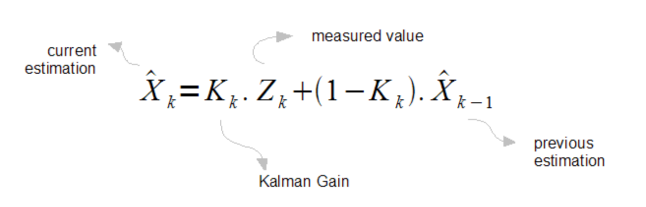
Note: The k's on the subscript are states (i.e. k = 1 ≡ 1[s], k = 2 ≡ 2[s], etc). The ^ symbol represents "the estimate".
KF is given by the state & measurement equations:
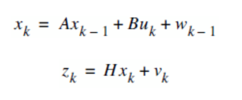
- xk is the signal value and can be evaluated by using a linear combination of the state, control signal and process noise.
- zk is the measurement value and can be evaluated by using a linear combination of the signal value and the measurement noise.
KF is a 2-step algorithm, the first one is the prediction (time update) step which is used to estimate the state of the system at the next time step, based on the previous state estimate and the system dynamics, and the correction (measurement update) which incorporates the actual measurements at the current time step, in order to refine the state estimate obtained from the prediction step.
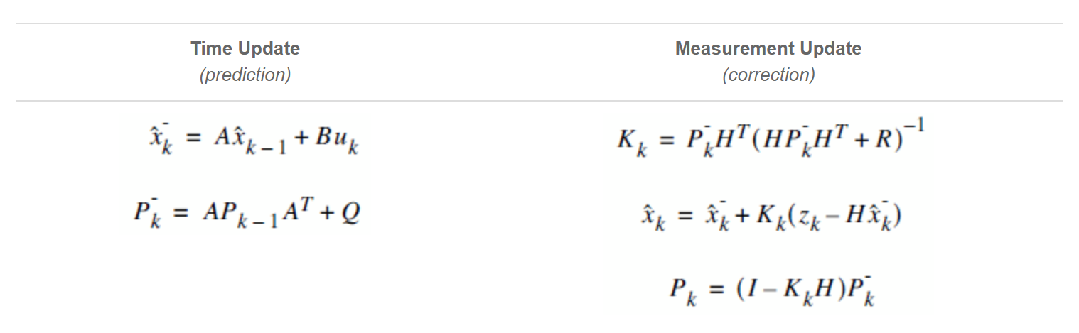
KF can be quite complex, for example: A, B, Q, H, R, P are matrices and each represents a part of the whole system. Generally its not easy at all to find those matrices (albeit some are easier than others), but luckly we can simplify it a lot, we just need to be a bit clever.
So lets do it!
- As every resource statistics is a single entity in our case, we have a 1-dimensional signal problem, so every entity in our model is a scalar, not a matrix.
- uk is the control signal which incorporate external information about how the system is expected to behave between measurements. We have no idea how the CPU usage is going to behave between measurements, therefor we have no control signal, so uk = 0.
- B is the control input matrix, but since uk = 0 this means we don't need to bother with it.
- A is the state transition matrix, and we established that we have a 1-dimensional signal problem, so this is now a scalar. Same as with uk, we have no idea how the CPU usage is going to transition, therefor A = 1.
- We just established that A = 1, and since A is a unitary scalar, this means AT which is the transpose of A, is AT = 1.
- Q is the process noise covariance matrix, it refers to unpredictable changes in the system that are not explicitly modeled. Guess what! That is going to happen all the time, but let's set it to Q = 0 (we'll revist it).
Following these assumptions, the prediction equations simplify to:
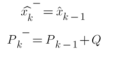
Which means that on each iteration, we will assign the prior estimate to the current estimate, and the prior error covariance to the current error covariance plus the process noise.
Lets continue our simplifications, now to the correction equations.
- Same as with the prediction, we deal only with scalars, not matrices.
- H is the observation matrix, which acts as a bridge between the internal model A, and the external measurements R. We can set H = 1, which indicates that the measurements directly correspond to the state variables without any transformations or scaling factors.
- Since H = 1, it follows that HT = 1.
- R is the measurement covariance matrix, which represents the influence of the measurements relative to the predicted state. We set this value to R = 1, which indicates that all measurements are assumed to have the same level of uncertainty, and there is no correlation between different measurements.
Following these assumptions, the correction equations simplify to:
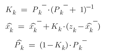
Which means that on each iteration, we will assign the prior estimate to the current estimate, plus the newly calculated kalman gain, times the difference of the measurement and the prior estimate.
Note: From now on, I will refer to error covariance by simply calling it error due to it being a scalar.
At some point this filter must "start" therefor we need to set values for the initial/prior estimate and error.
- xk-1 = 0 - Means that we are starting blank, there is no prior estimate.
- Pk-1 = 1 - Means we have practically zero trust (as we should so) on the initial state.
Addressing Requirements and Signal Characteristics
- For the rest of this article, all blue-colored signals represents i(n) (raw signal) and the orange-colored ones are o(n) (filtered signal).
- All i(n) signals are computer simulations of various CPU usages and trends, they don't represent actual measurements.
- I am aware that some of the signals shown in the rest of this article, aren't your typically CPU usage patterns. But they are edge cases which are interesting to talk about and are crucial for the analysis and modeling of the filter.
- The number of iterations on all signals in the charts is fixed to 2500 which is a dimensionless unit. The frequency of sampling does matter! But when representing 1 day with 2500 data-points, we shall see that it is enough to represent the original signal (albeit in a transformed form). In addition, the default frequency of sampling is every 1 second, which translates to 86400 data-points within a timespan of 1 day, which further strengthens the trustworthiness of the filter.
Requirement 1
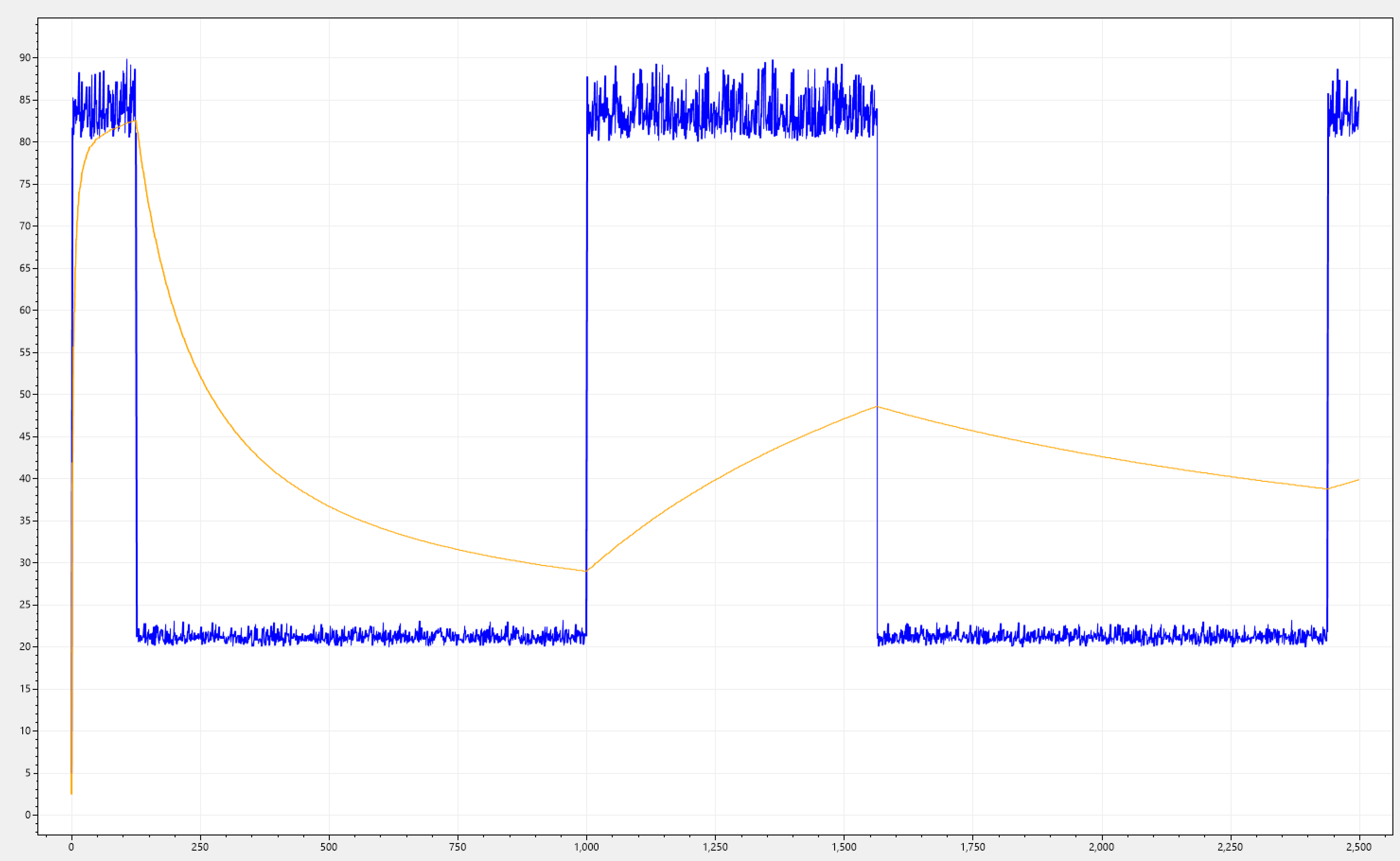
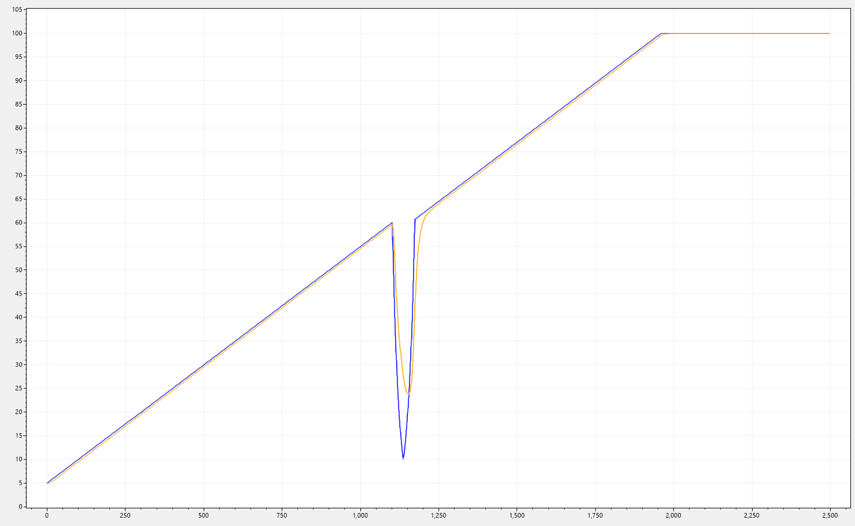
Let's have a look at the chart below. i(n) increases steadily but has a sudden fluctuation which occurs at the 60% mark. It suddenly drops all the way to 10%, and jumps back to 60%. It all happens within a narrow window representing 3% of the total execution time.
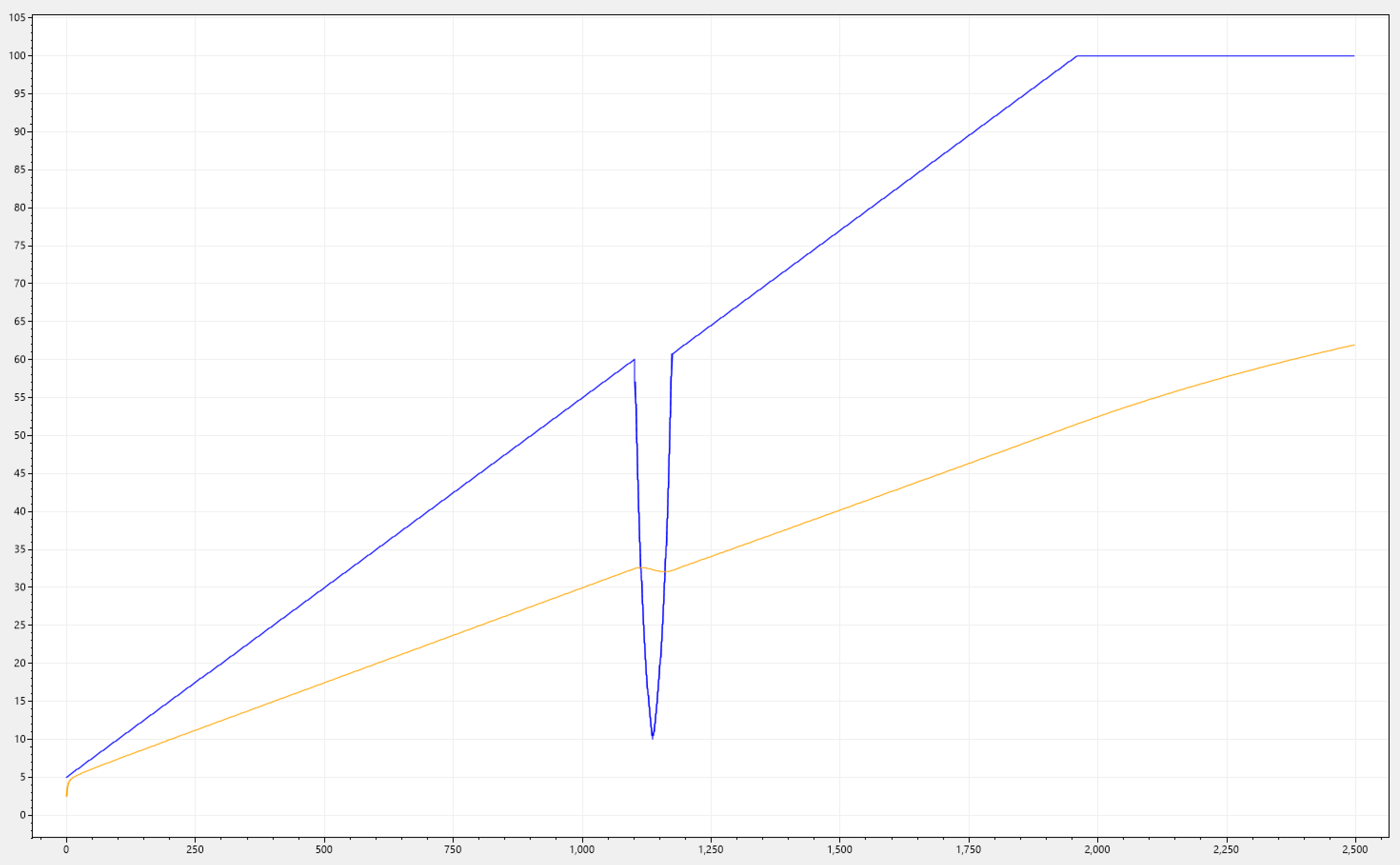
Imagine now a series of placement decisions being made, right in-between this drop. This silo would be considered very underloaded, and there is potential for an influx of activations comming to this silo. But we can see that the workload has not finished, there was just a stall which could have been an I/O operation that needed some additional data for the currently executing logic. Once it would pick up, it would find itself in an overloaded silo now, due to the new activations.
Note how o(n) performs a great deal of damping. But how did we managed to achive this?
Remember that we set A = 1, this is the state transition matrix (scalar in our case) this has a smoothing effect and acts like a low-pass filter. This is hugley contributed to A = 1 as the model assumes no inherent dynamics or natural tendencies for change in the system's state. We also have set R = 1, this is the measurement convarance matrix, meaning that we distrust the measurements a lot. Overall its like gently pulling the predicted value towards the previous one, making it less prone to sudden jumps or fluctuations. Basically the system has a great deal of inertia.
Below you can see different simulations, all sharing the same effect.
Packed with this knowledge let's revisit our requirement, which stated:
Given any kind of signal-drop in i(n), than o(n) must follow a trajectory that decays with a slower rate than that of i(n).
o(n) certainly follows a trajectory that decays with a slower rate due to the high-frequency component filtering, but due to the inertia introduced, we made things way worse when it comes to tracking i(n) when there is a signal rate increase (which in this case its like 97% of the whole spectrum). Which bring us to the next requirement.
Requirement 2
With the satisfaction of requirement 1, we introduced the problem of tracking i(n) when there is a signal rate increase. Let's address this now!
Remember how the process noise covariance Q, refered to unpredictable changes in the system that are not explicitly modeled. We set this initially to Q = 0, which meant that we don't expect any unpredictable changes in the system, and as mentioned above, this is not the case as we will have unpredictable changes all the time! Increasing this value will tell the filter to account for uncertainty.
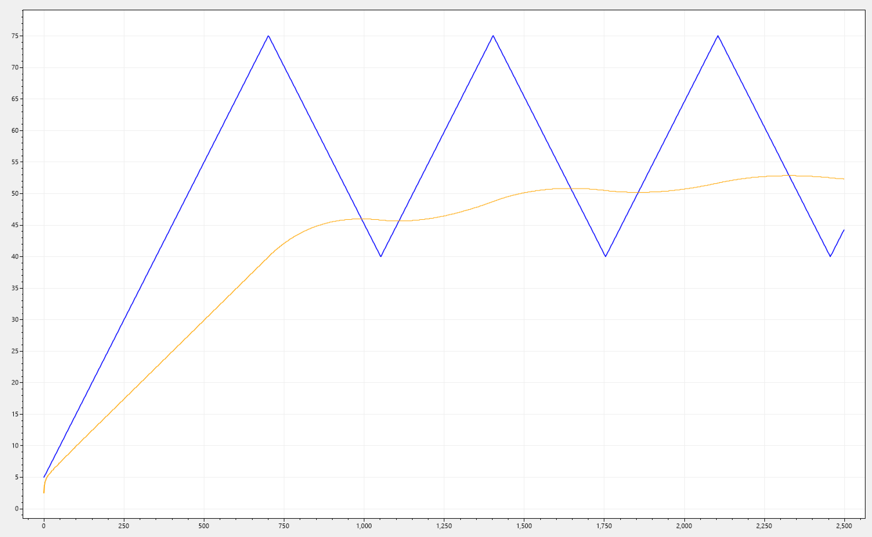
Below we can see the same graph as above, but instead of just having i(n) and o(n), we are showing 3 different filtered signals, each having a different value for Q. Note that by increasing Q, the signals ok(n) track i(n) faster and faster, but at the price of less damping!
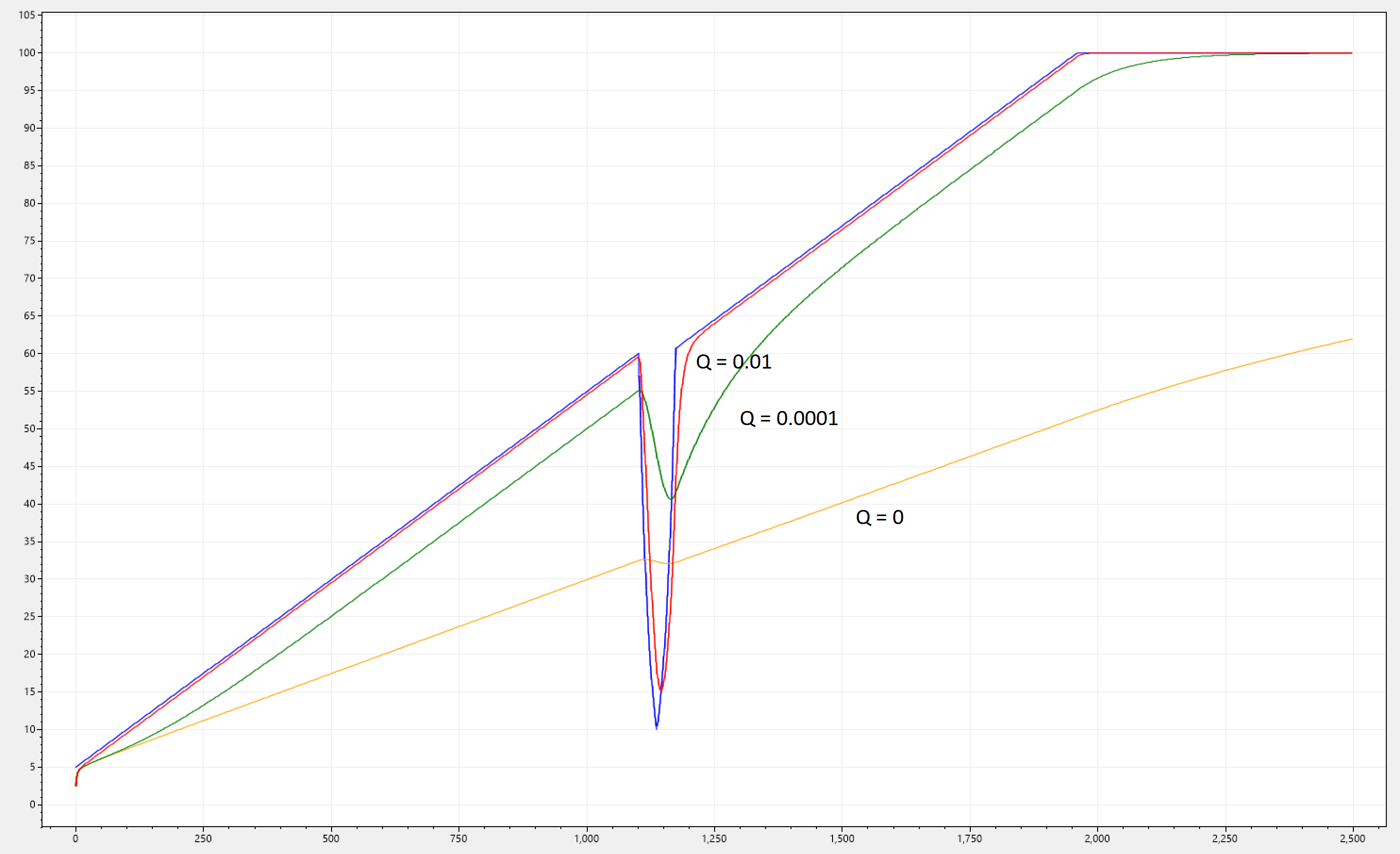
Packed with this knowledge let's revisit our requirement, which stated:
Given any kind of signal-jump (especially rapid once) of i(n), than o(n) must follow those as fast as possible, yet still provide some level of damping to avoid skewing placements due to miniscule fluctuations in the statistics.
The requirement is statisfied, and although technically the best value for fast-tracking would be Q = 1 (expect unpredictable changes all the time), we want to preserve some level of damping, therefor we will stick with Q = 0.01.
Dual-mode KF (DM-KF)
It should be clear by now that requirements 1 & 2 are inversely correlated to each other. The better we fix one, the broken the other gets!
In order to overcome this issue, we stick with the values of KF that work for each case, and sepparate the responsibilities into two KFs. These two filters will be combined into a single one, which operates in two modes: slow (SKF), and fast (FKF). The only differentiating factor between them is Q; where QSKF = 0 and QFKF = 0.01.
While we want to switch between SKF and FKF, it is important that we run both of them at each iteration, this is because if we just switched whenever the measurement is greater than the estimate of SKF, eventhough FKF is fast, it would still be lagging behind. Much the same way when a transition of type FKF -> SKF happens, SKF will lag behind. Different from SKF -> FKF, the transition FKF -> SKF would be way more noticeble, due to the inert nature of SKF.
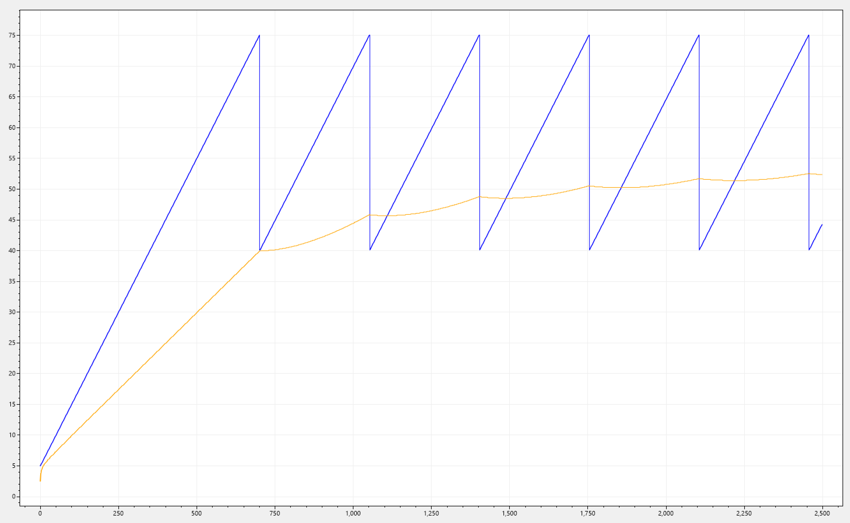
Let's showcase this in action by using one of the signals we showcased above.
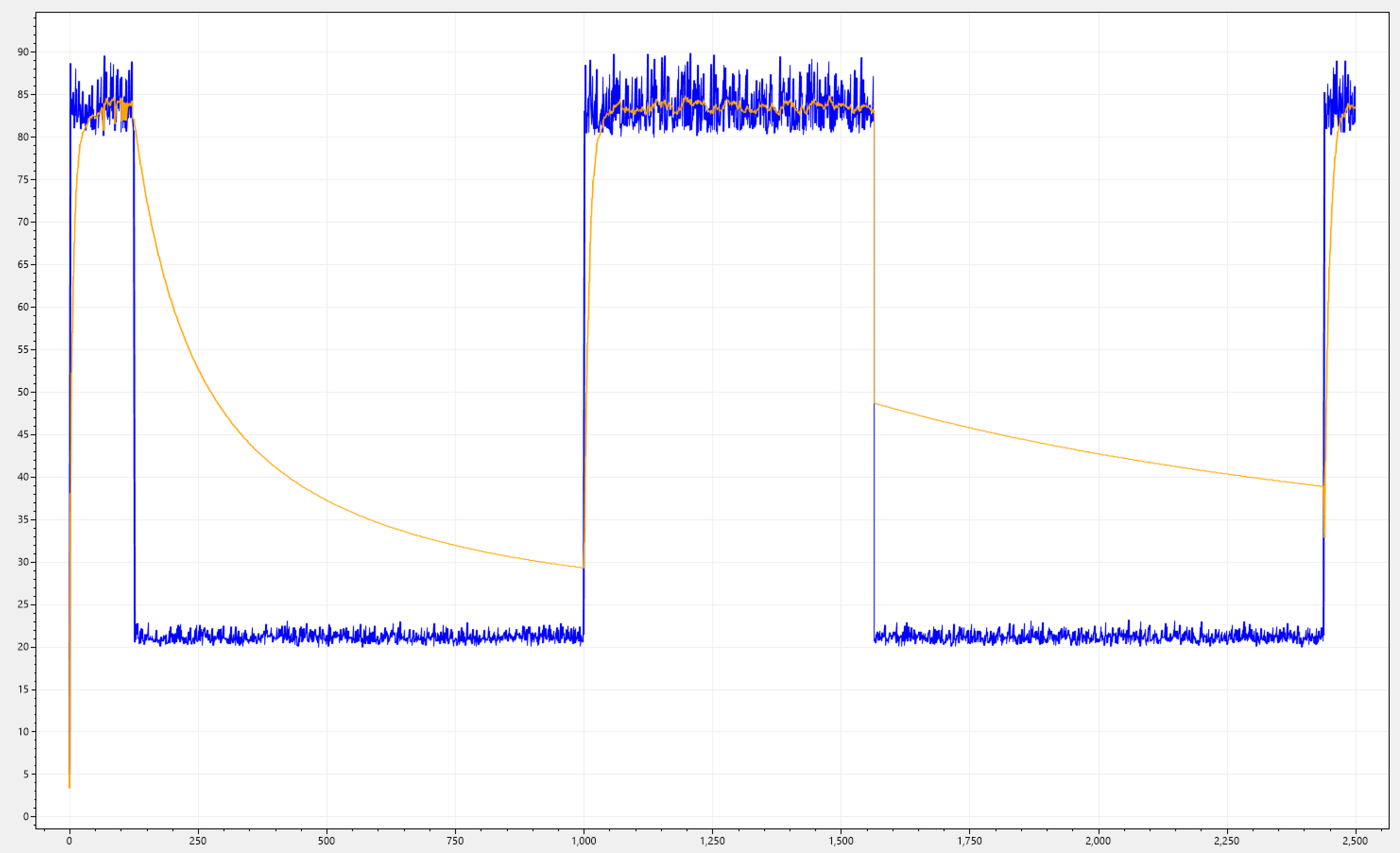
Ahh, much better! Notice how FKF takes over right at the begining and tracks i(n) very fast, then SKF takes over and provides a slower decay rate. This is exactly what we wanted!
But hold on for a second? This seems to work great at the begining, but notice in the second signal-drop how o(n) quickly jumps down to around the middle and then progresses with a slower rate.
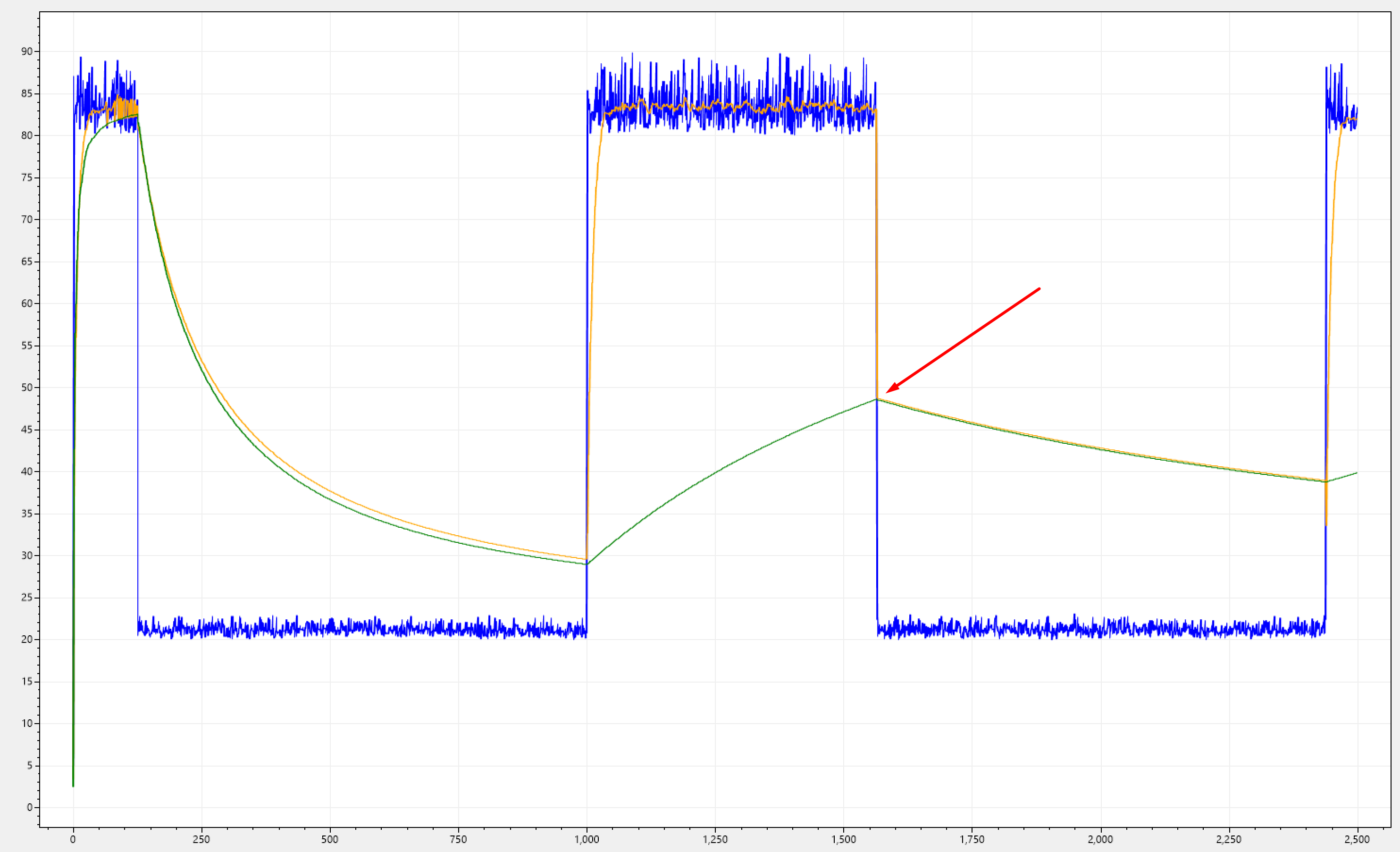
Below I have overlapped both filtered signals: single-mode KF (green), and DM-KF (orange). Notice how the amplitude (where the red arrow points) of this down-jump matches perfectly with our single-mode KF.
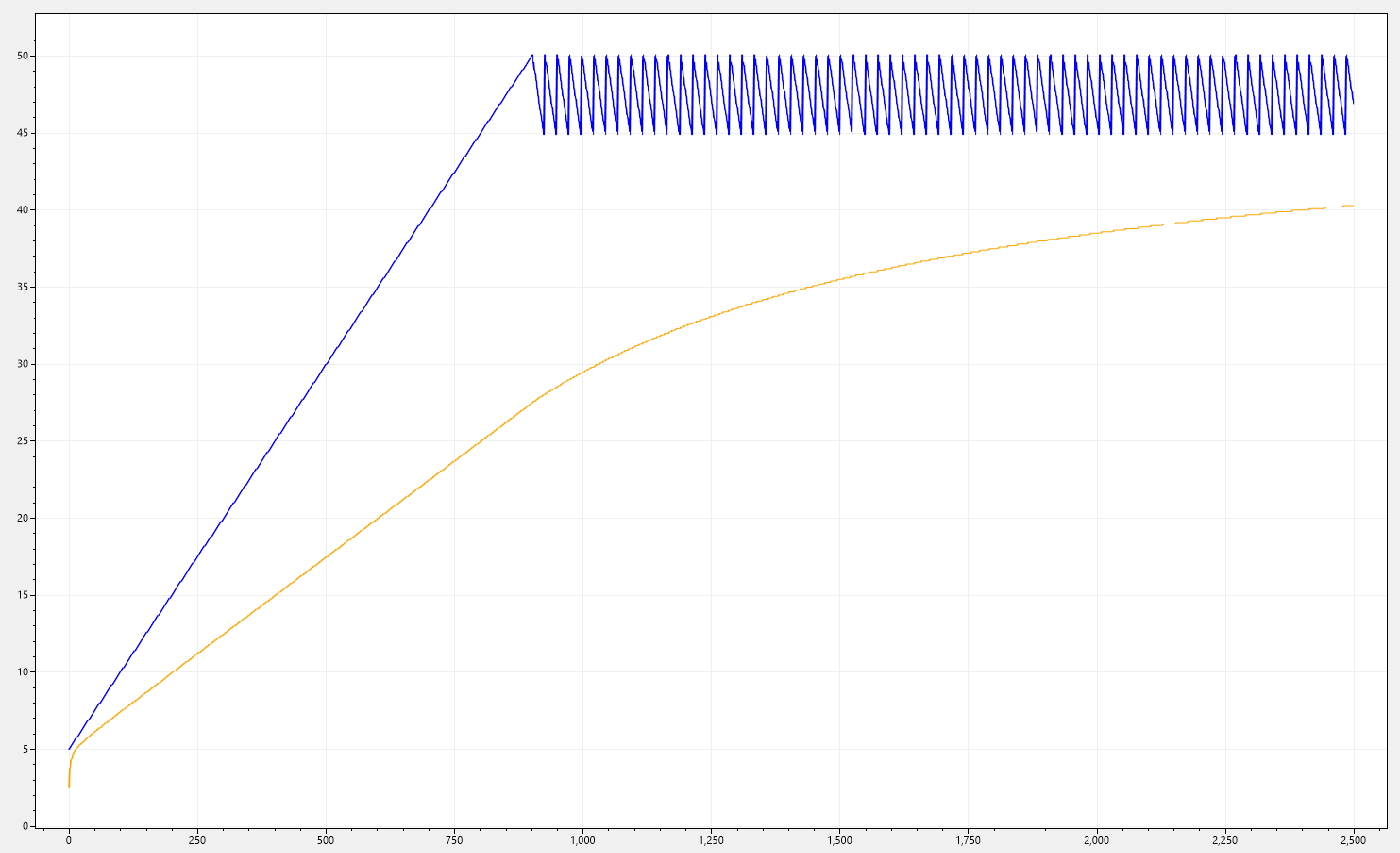
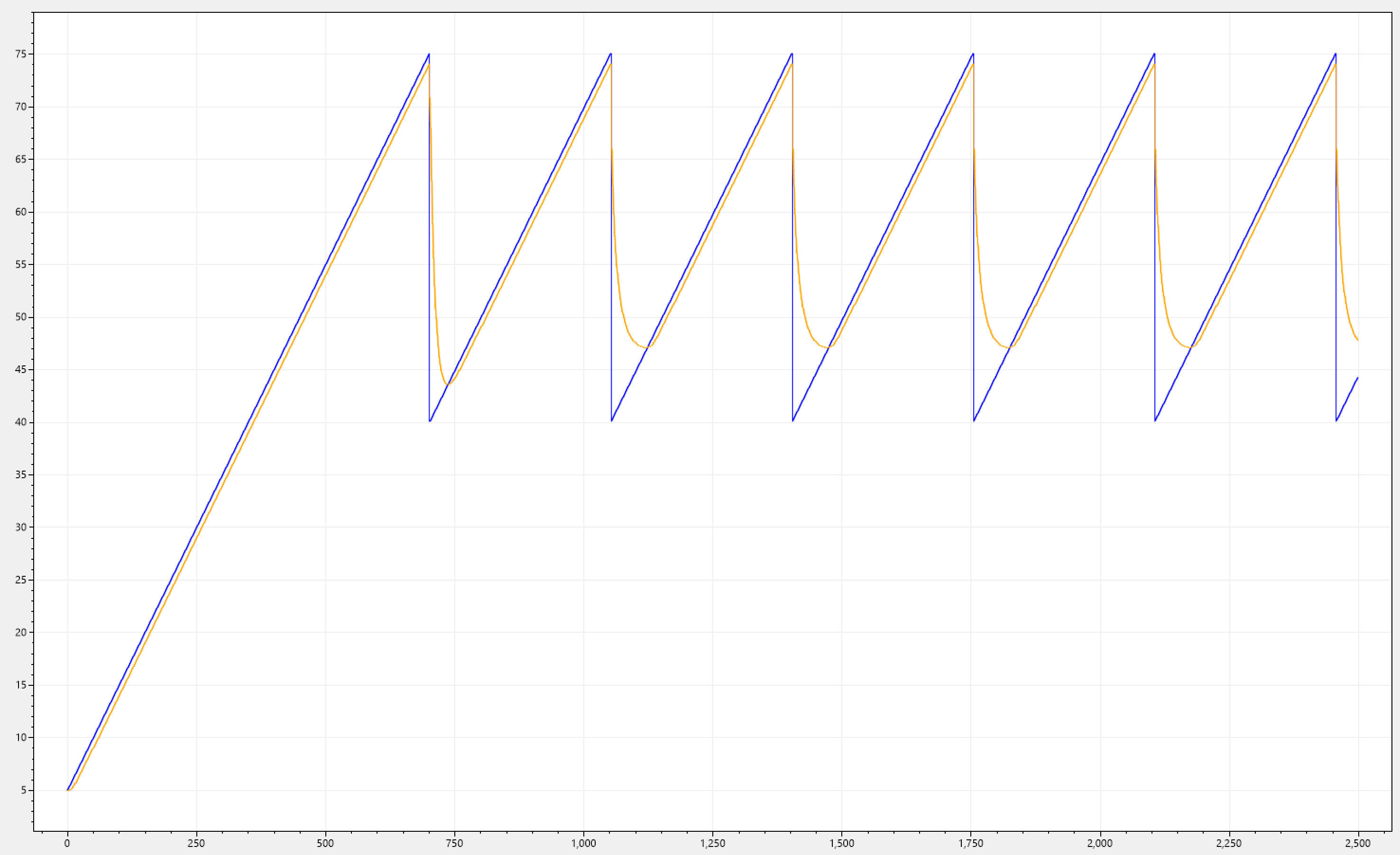
Let's pick a different signal that has a higher frequency over the same iterations, so we can observer that this behaviour is not just a fluke, but instead represents an accumulation problem.
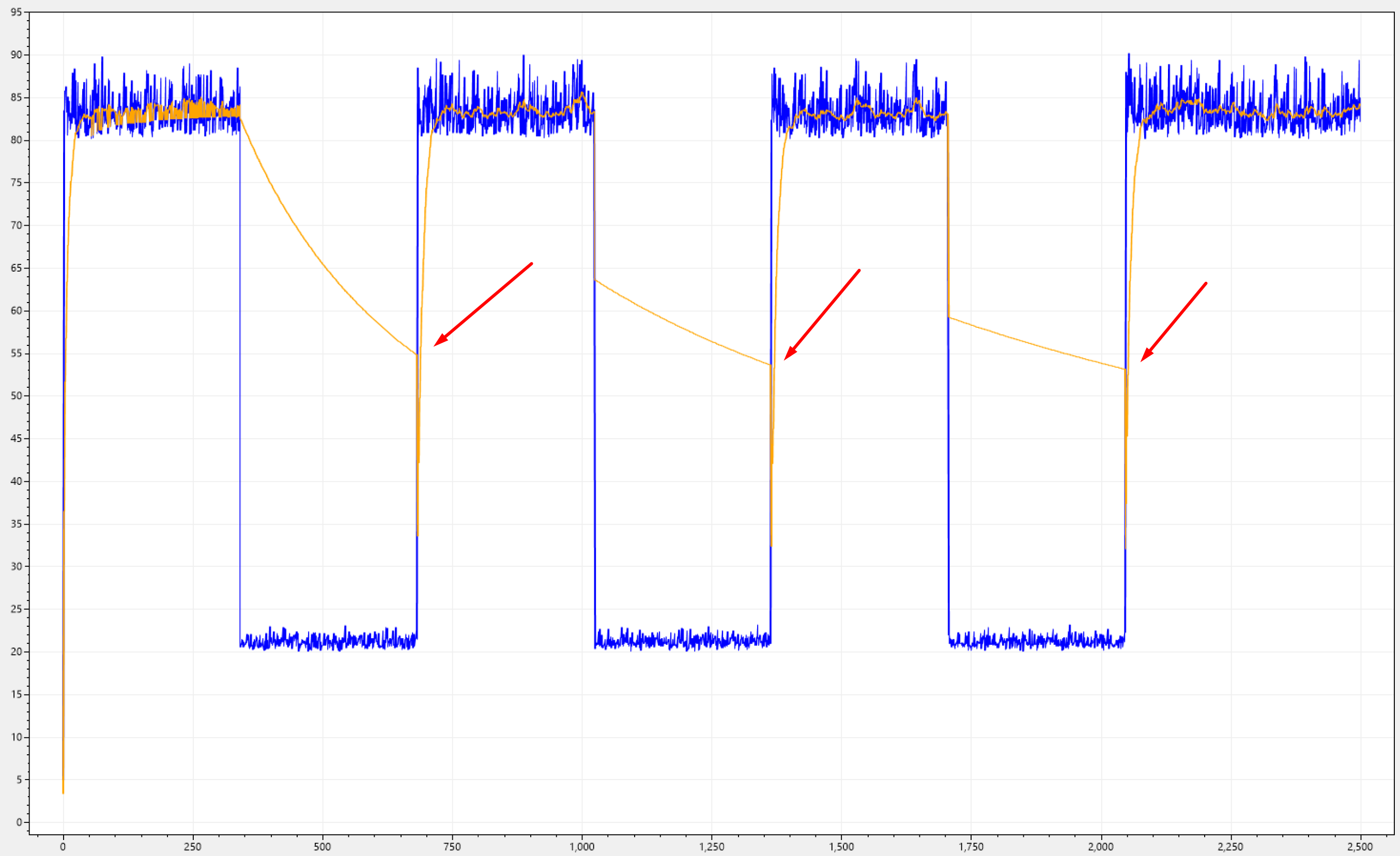
It's clearly visibile that SKF will converge towards the avarage of the whole signal, and its expected becuase the error will accumulate over time, this leads to a gradual reduction in the kalman gain, making it less responsive, resulting in a more linear response. Too linear though!!!
When a placement is about to happen, the filter will consistently report too much stress on the silo, which it's not the case. Our goal is not to underutilize the silo, but instead to avoid overloading it to quickly.
This tells us that there is more to it than simply running both filters independently and switching between them. What we need is them to cooperate.
In order for them to cooperate, upon switching from FKF to SKF, we need to update the state of SKF so that it has information on where FKF left-off before the switch. We do so by setting the current estimate of SKF to be equal to the current measurement, in addition we need to reset the current error to 0, indicating that we want to fully trust the measurement in order to reflect the actual signal's value.
In the otherhand, upon switching from SKF to FKF, and due to SKF accumulating the error, we need to reset its state so that it aligns with the current peak of FKF, so that we get a slower decay that is always aligned with the latest FKF state, and not the overall state of the whole signal over it's lifetime.
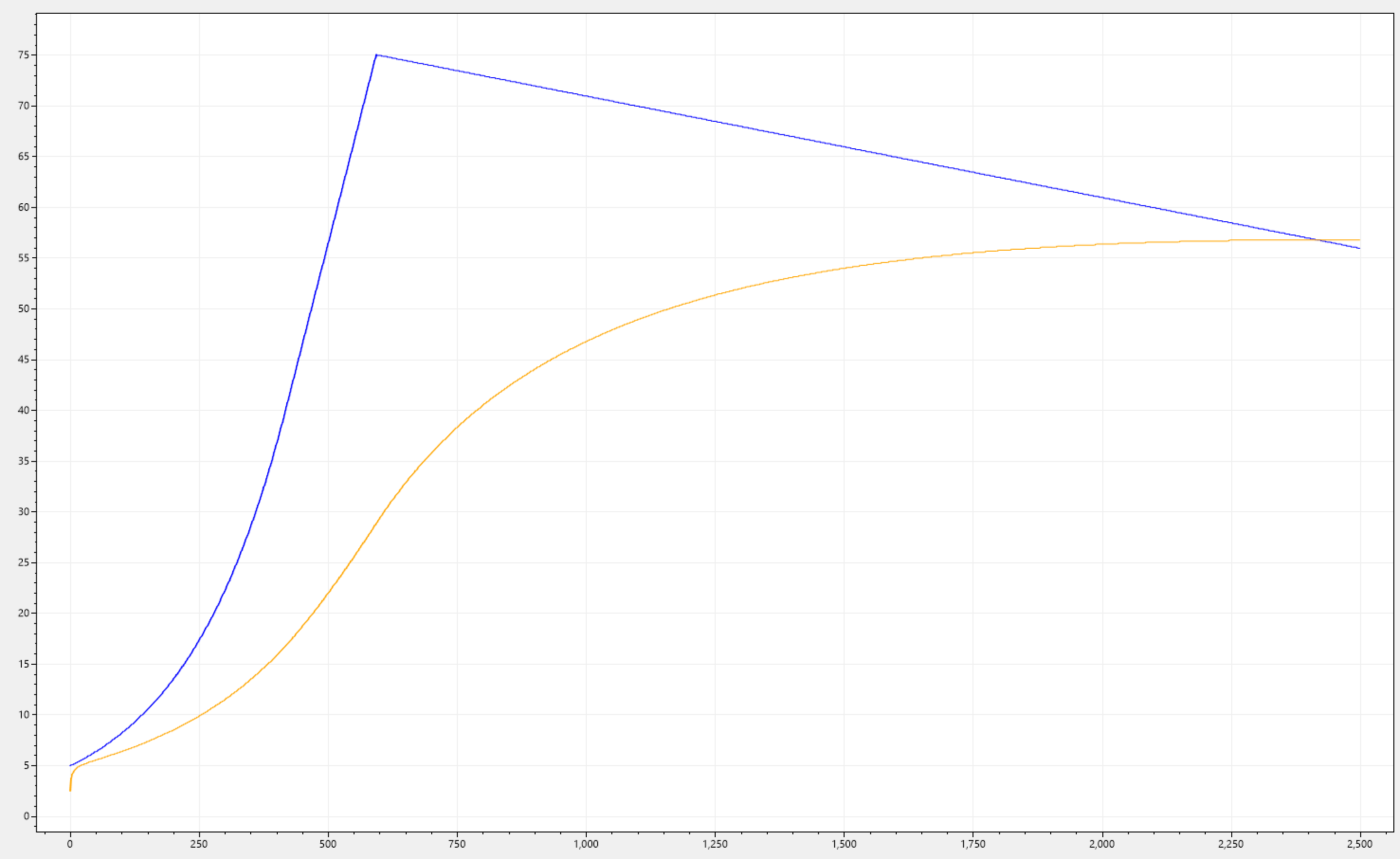
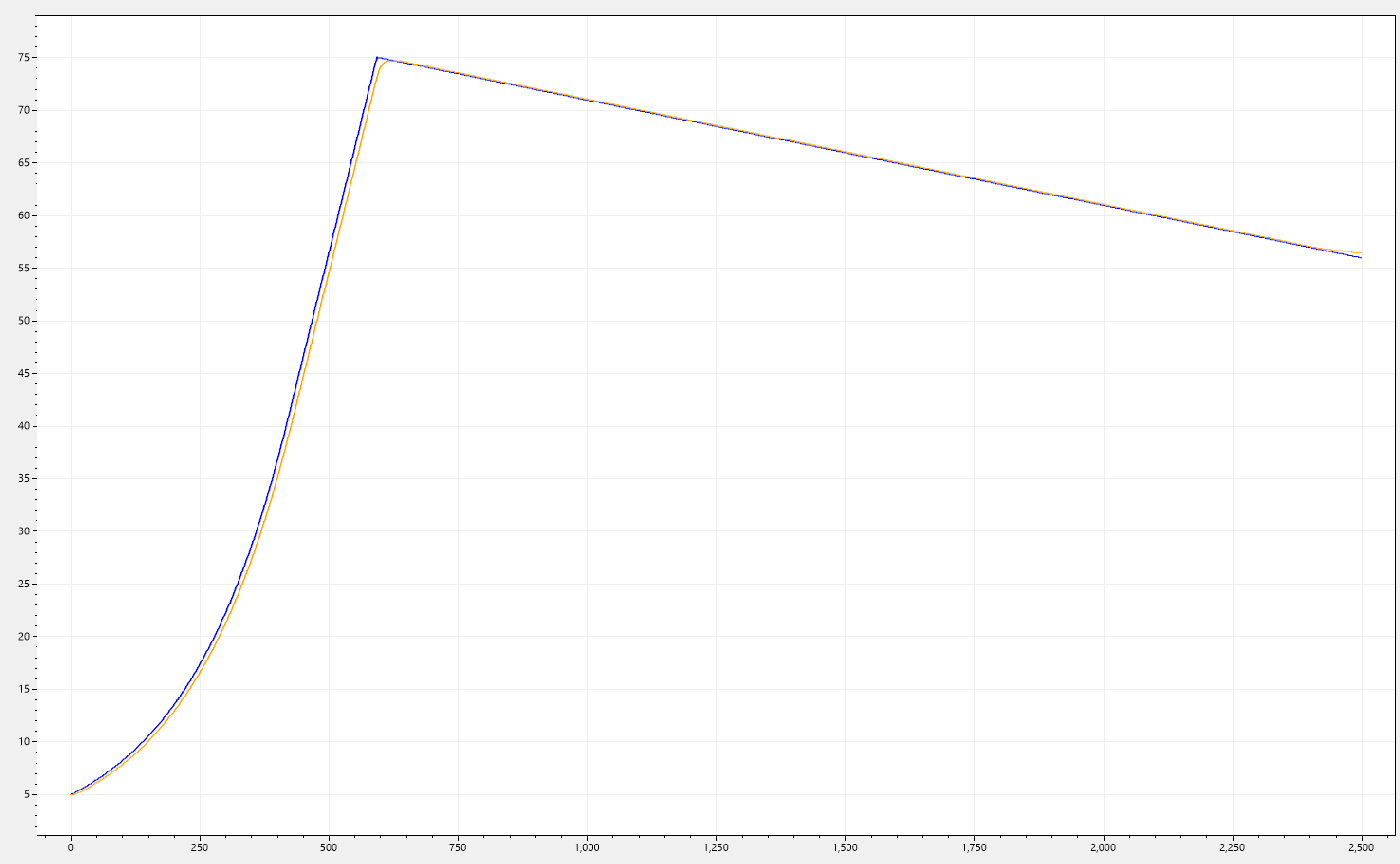
After we perform these changes we can observe a much better response. We can see that with the cooperative DM-KF (CDM-KF), we managed to statisfy both requirements 1 & 2, without them impacting each other.
The CDM-KF acts as peak detector on the way up, and as a low-pass filter on the way down. The regime switching ensures:
- No stale state.
- No lag on spikes.
- No jitter on decay.
- No discontinuities.
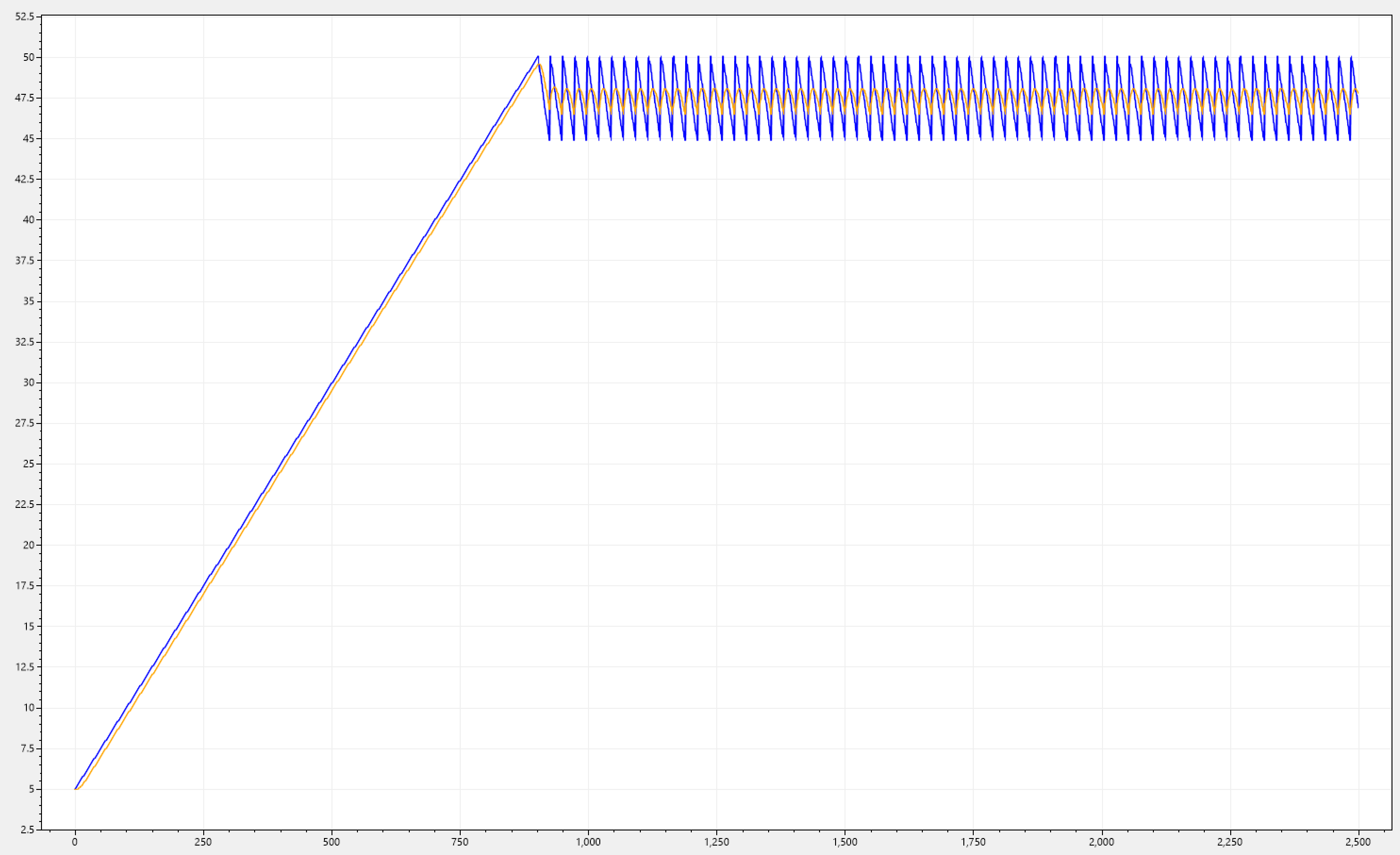
One interesting thing to note is that in the very first crest of the wave-like signal i(n), we can see that FKF is ever so slightly slower to catch up, as opposed to the next set of crests. The same is true for SKF, it is slower to decay and than quickly stabilizes.
For both cases, this is due to the initial estimate of both filters being 0, because when the program starts, we don't have any prior knowledge of the system (in terms of measurements), so they both need to do some "trial & error" till they approach the actual signal.
In the case of SKF, this startup behaviour is actually desirable, because we want to provide a view to the placement director that this 'new' (being an actually new, or restarted) silo, is under more load than in actually is, since we can avoid overloading it before it starts properly operating. Typically this is the time when the silo is the most vulnerable for overloading.
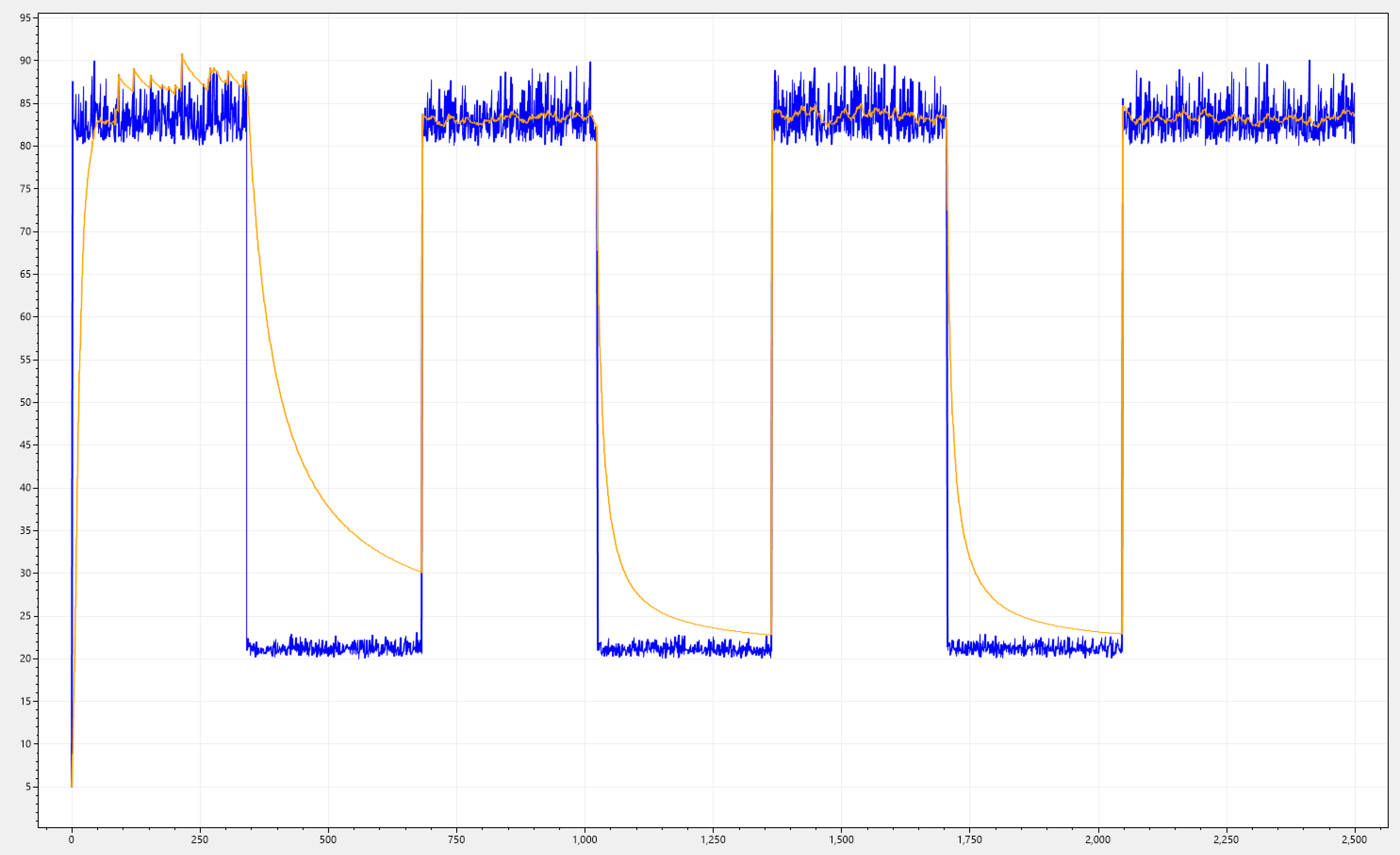
Below we can see CDM-KF applied to our initial signal trends. This is for the sake of completeness, and showing that the filter works consistently across.
Requirement 3
KF (therefor by extension our CDM-KF) is an recursive algorithm, so it can operate just by keeping the values of the prior iteration only. From a memory consumption aspect, other than the allocated memory for the filter object itself, there are no additional memory allocations.
The filter is also conservative in the processing aspect. Below we can see two benchmarks that assign 1000 measurements vs running them through the filter and afterwards assigning them.
| Method | Iterations | Mean | Allocated |
|---|---|---|---|
| AssignMeasurements | 1,000 | 861.3 ns | - |
| FilterThanAssignMeasurements | 1,000 | 12,052.1 ns | - |
The benchmarks tell that on avarage the computational needs for running a measurement through the filter is ~12 [ns]. While its true that if we do not run it through the filter, the time will be quite smaller, we need to keep in mind the context under which this will run.
The default period of statistics collection is 1 [s], so the filter theorically could process a total of ~83 million measurements, which fully statisfies the requirement for the algorithm to complete within the bounds of the sampling period chosen.
Unless the period is chosen to be under ~12 [ns] (which would mean bombarding the management grain), we are totally fine. What we are doing is essentailly we are utilizing a fraction of the idle time that would be between two subsequent measurements.
Packed with this knowledge let's revisit our requirement, which stated:
The solution must be conservative on resources, and must complete within the bounds of the sampling period chosen.
The requirement is statisfied!
Clearing the Fog
If you've made it this far, and you approached this article with a healthy dose of scepticism, there might be a thing floating in your head that may make you uncomfortable. Let me address it for you, in case you are (rightfully so) confused.
If this algorithm is applied to all silos in a cluster, it will work consistently across all of them. It may seem that regardless wether the algorithm was applied or not, they all will get damped with the same rate, so the underlying K-choices algorithm will pick the same silo as it would before. But that is not true! Let's analyze this via the diagrams shown below.
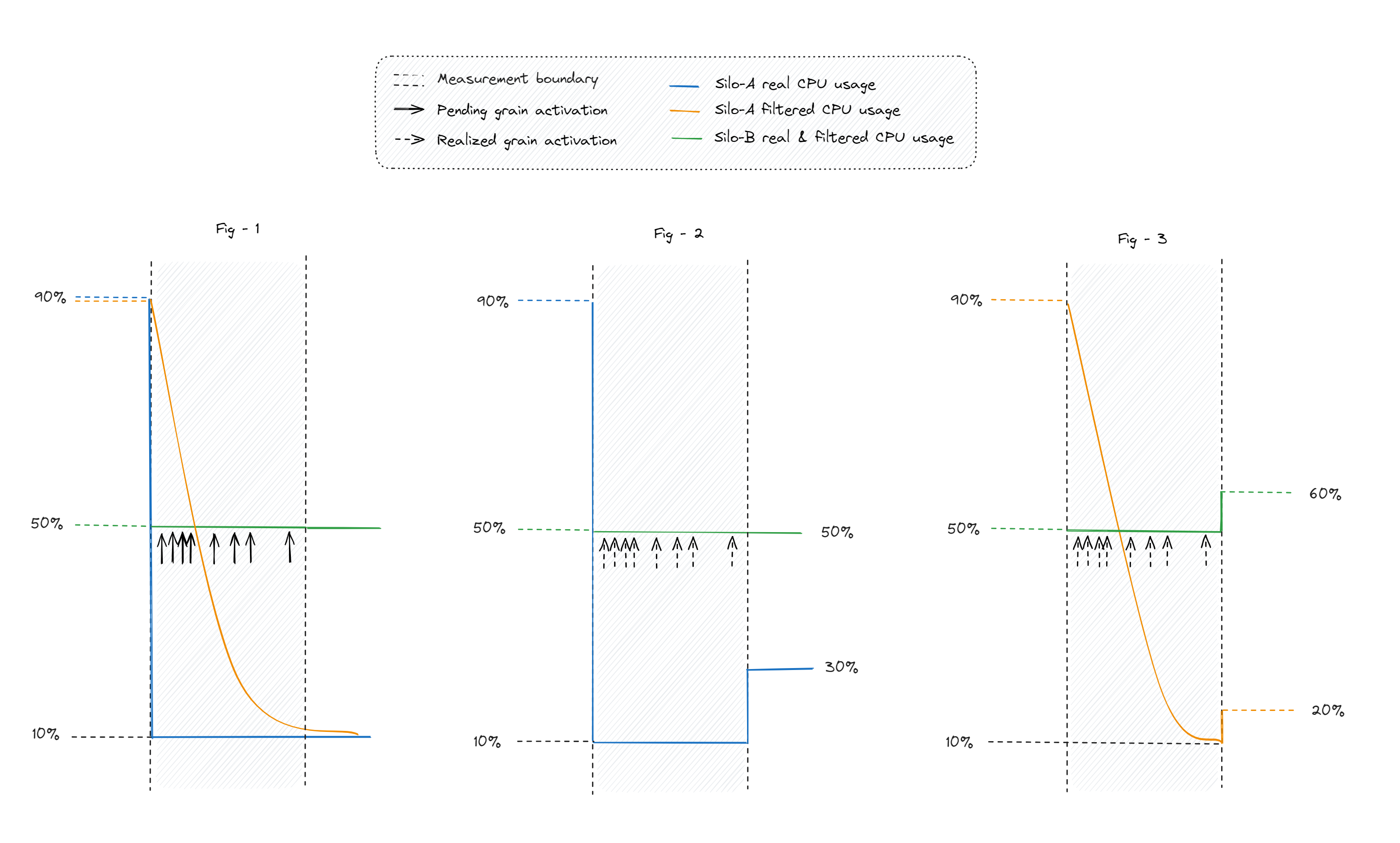
- In fig 1, we show three signals (see legend), this is the starting point.
- In fig 2, CDM-KF has not been applied therefor after the measurement boundary has elapsed, silo A will find itself at 30% load (a bump of 20%), and silo B will stay at 50% (no bump).
- In fig 3, CDM-KF has been applied therefor after the measurement boundary has elapsed, silo A will find itself at 20% load (a bump of 10%), and silo B will also jump, this time at 60% (a bump of 10%).
Sharing the load between the two silos is better than all going to a single one. Not just from an overloading prespective, but also from an utilization prespective. If each silo has dedicated resources, than it would be good if we utilized them.
Summary
- While this article was geared towards Orleans and silos, everything that has been discussed can be used to enhance resource-based load-balancing algorithms in a cluster of servers.
- We saw how to apply an algorithm from control theory (KF) to a computer science problem.
- We understood how KF operates, and created our own version CDM-KF.
- We have used CPU usage as the resource indicator, but this can be easily extended (and has been) to RAM, and theoretically to activation-count placement in Orleans.
Overall the solution provided us with the following benefits:
- Enhanced Stability - Dampens load fluctuations by reducing abrupt changes that could overload individual silos.
- Proactive Load Management - Anticipates potential overload scenarios to early signals of increasing load, and preventes reactive measures.
- Handling of Transient Overloads - Filters out short-term load spikes, allowing silos to naturally recover without triggering immediate placement change decisions or load-shedding actions (in case live grain migration is used).
- Reduced Oscillations - Prevents rapid oscillations in load distribution that could occur with an overly sensitive load-balancing mechanism.
If you found this article helpful please give it a share in your favorite forums 😉.
The solution project is available on GitHub.