

Introduction
Cache invalidation and replication are notoriously difficult problems in distributed systems. Traditional approaches often rely on centralized leaders, pub/sub message brokers, or naive broadcast protocols that scale poorly and flood the network. Replicating state globally usually means either high communication overhead or intractable computation bottlenecks.
This article explores a radically different approach. Leveraging Rateless Invertible Bloom Lookup Tables (R-IBLTs) and the distributed actor framework Microsoft Orleans, we can build a leaderless, epidemic gossip protocol that achieves low-overhead, zero-hop cache memory reads. We will break down how we encode memory differences into an infinite streams of symbols, allowing any node to synchronize with any peer in such a way that its nearly optimal to the theoretical limits.
The Bloom Filter
Before we dig deeper, lets start with the data structure that kicked off this whole thing. A Bloom Filter is a space-efficient probabilistic data structure used to test whether an element is a member of a set. It consists of a simple bit array initialized to 0's. When inserting an item, the item is hashed by k different hash functions. Each hash function produces an index, and the bit at that index is set to 1. For example, hashing the item x with 3 hash functions, yields indexes [0, 2, 4].
The hash space is the space of all possible results the hash function(s) can produce a value in. The filter lives and operates on that space of hash results.
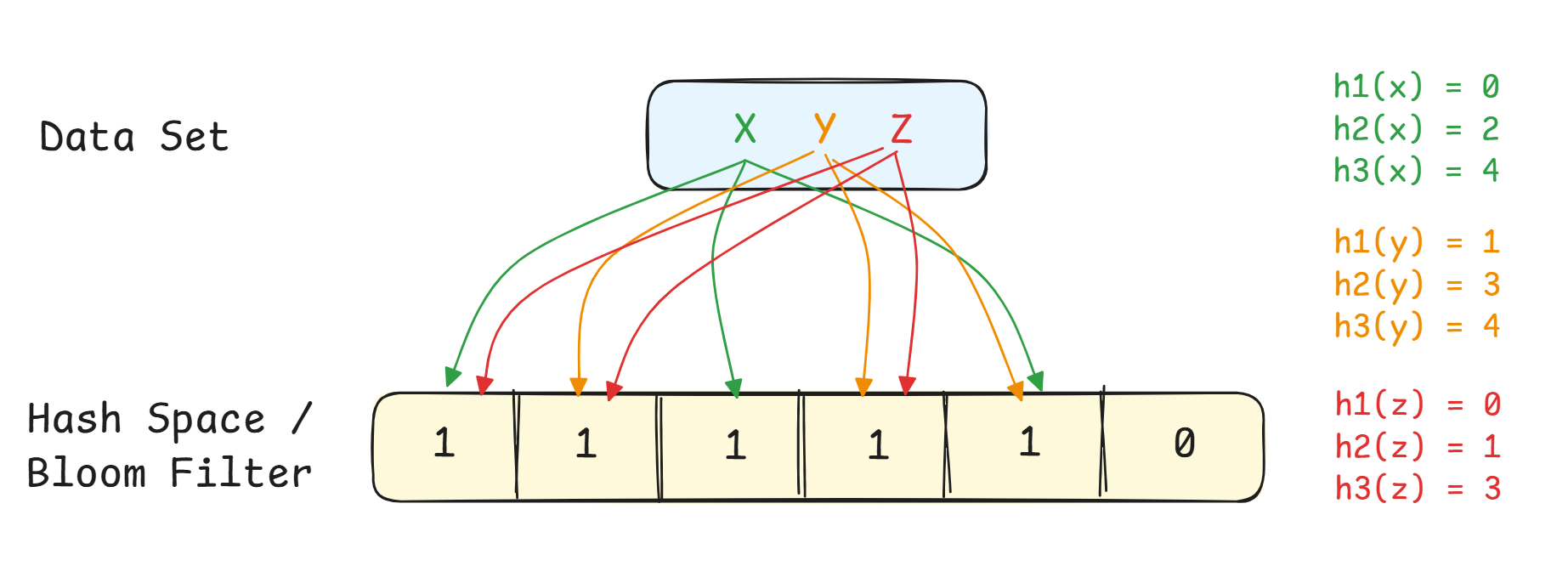
Given we have the filter with the above state, if we check for presence of items [x, p, r] the filter can answer with "definitely not in the set", and "maybe in the set".
If we check for the presence of item x, we run x through the same hash functions, which yields the indexes [0, 2, 4], all bits at those indexes are 1, which means the filter will say "maybe", reality is that it is in the set.
If we check for presence of a new item p, we run p through the same hash functions, which yield indexes [1, 2, 4], all bits at those indexes are 1, which means the filter will say "maybe", reality is that it is NOT in the set.
If we check for presence of a new item r, we run r through the same hash functions, which yield indexes [0, 3, 5], NOT all bits at those indexes are 1, which means the filter will say "definitely no", reality is that it is NOT in the set.
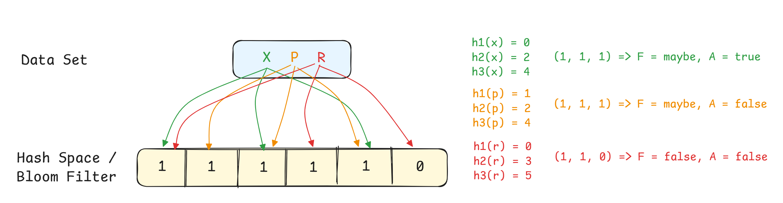
With r, we got a "definite NO" since the index at h3(r) = 5 is 0, so the filter can guarantee that r is NOT in the set.
With p, we got what is a called a "false positive", the filter said that p maybe in the set, but we know from the insertion step, we never inserted p, it just happened to be that the indexes: [1, 2, 4] correspond to the hash results [h1(y) / h2(z), h2(x), h3(y)].
It is possible to tune this false positive rate and bring it down as much as we like (not 0% though), but that comes at the expense of having to use more bits-per-element which increases the memory footprint, but also it means we have to use more hash functions, which increases the CPU overhead.
While incredibly memory efficient, standard Bloom filters have a critical limitation in that you can not remove, nor list items currently inside them.
Invertible Bloom Lookup Tables (IBLTs)
Say server A has a set {x, y, z} and server B has {y, z, p}, the act where both servers end up having the set {x, y, z, p} is called set reconciliation. One way for the 2 (or any number) servers to reconcile their sets is for each of them to transfer their set to each other and calculating the difference. It should not come as a surpise that this would become infeasible for large sets, and very inefficient too!
The Bloom filter we discussed above would be an efficient way to do so, since it encodes the local servers' set, unfortunately as we elaborated above we can not extract the encoded elements from the filter itself, as the INSERT operation on Bloom filters is a fundamentally destructive operation. This is where IBLTs comes into play!
While Bloom filters only store 0's and 1's in each of the hash space cells, IBLTs store additional data in each cell, which subsequently allows "peeling" out the actual values from the filter itself.
Note that IBLTs work on a
(key, value)pair basis, not just a "presence" bit basis as do regular Bloom filters. We will refer to the bitwise exclusive OR operation using the ⊕ symbol.
An IBLT cell is composed from these field:
KeySum - The ⊕ of all the keys (unique identifiers) that have been mapped to this specific cell by the k-hash functions. When a new item is inserted, its key is ⊕ against the current state of this field. Because ⊕ is its own mathematical inverse, removing a key uses the exact same ⊕ operation, naturally erasing its presence from the sum.
ValSum - The ⊕ of all the values associated with the keys mapped to this cell.
CheckSum - The ⊕ of all the hashes of the keys that have been mapped to this specific cell.
Count - A signed integer that tracks the net total of items currently mapped to this cell. It increments by 1 for every insertion, and decrements by 1 for every deletion.
Having these fields is what allows IBLTs to support the LIST operation, which is what is needed for reconcilliation. The peeling process works by scanning the array for "pure" cells. A cell is considered "pure/decodable" when 2 conditions are met:
Count is exactly 1 (indicating the local server is missing an item which is present on the remote server), or -1 (indicating the local server has an extra item which is missing on the remote server). Though this can be flipped depending on the convention used.
The hash of the KeySum exactly matches the CheckSum, formally Hash(KeySum) = CheckSum. With high probability the count check should be enough, but checksum check confirms that the recovered key is consistent with the accumulated fingerprint. Without this, a cell could (albeit with negligible probability given a large fingerprint such as 64/128 bits) falsely appear to contain a single key due to ⊕ cancellations (or just data corruption).
Once a pure cell is identified, the exact key and value can be extracted directly from the KeySum and ValSum. The peeling process (also refered to as a the 'peeling decoder') then takes that extracted item, hashes it again to find the other cells it was mapped to, and actively ⊕'s it out of those cells while decrementing their Count field. This artificially removes the item from the rest of the table, often revealing new pure cells and creating a cascading avalanche effect that entirely reveals the set difference.
In short, the overarching idea is that one side of the parties looking to reconcile their datasets, first compacts their current state into an IBLT, than sends it over the network to its peer.
Upon receiving the remote payload, the peer ⊕'s its local IBLT against the received one. Because of the mathematical properties of ⊕, any data shared by both nodes cancels itself out to zero. What remains is a functionally distinct IBLT that represents the exact mathematical set difference (Δ) between the two servers. It is from this IBLTΔ that the peer begins the peeling process to extract the conflicting keys.
Beware that the peeling process (the LIST operation) is in itself a destructive operation, meaning that the contents of the IBLT are actively consumed and zero'ed out as the items are sequentially extracted. If you need to retain the structural state of the IBLT after the extraction completes, you must explicitly create an in-memory copy before you begin peeling.
In the world of distributed systems, this is generally not an issue to begin with, since sharing state with a remote peer inherently requires serializing the IBLT payload over the wire. Consequently, the receiving node is already working with a deserialized copy of the remote IBLT. This network copy can be safely mutated and completely destroyed during the decoding phase without ever impacting the underlying cache state or original IBLT of the sender.
Encoding
When I refer to an item such as x, y, z, it is meant to be the keys of these items, and with them the associated vx, vy, vz values. I will also skip the CheckSum along these exercises.
Assume we have a 7-cell IBLT and k=3 hash functions. First, we insert item x. Our hash functions map x to cells 1, 2, and 3. We ⊕ the key x into the KeySum, the value vx into the ValSum, and increment the Count.
| Cell 0 | Cell 1 | Cell 2 | Cell 3 | Cell 4 | Cell 5 | Cell 6 | |
|---|---|---|---|---|---|---|---|
| KeySum | 0 | x | x | x | 0 | 0 | 0 |
| ValSum | 0 | vx | vx | vx | 0 | 0 | 0 |
| Count | 0 | 1 | 1 | 1 | 0 | 0 | 0 |
Next, we insert item y. Our hash functions map y to cells 2, 3, and 4. Notice how the overlaps in cells 2 and 3 are handled by the ⊕ operator, and the counts on the same cells is 2.
| Cell 0 | Cell 1 | Cell 2 | Cell 3 | Cell 4 | Cell 5 | Cell 6 | |
|---|---|---|---|---|---|---|---|
| KeySum | 0 | x | x ⊕ y | x ⊕ y | y | 0 | 0 |
| ValSum | 0 | vx | vx ⊕ vy | vx ⊕ vy | vy | 0 | 0 |
| Count | 0 | 1 | 2 | 2 | 1 | 0 | 0 |
This process repeats until the entire dataset is encoded. This compacted, probabilistic data structure is what gets serialized and sent over the wire.
Decoding
To understand how to list the elements out of an IBLT, we look for pure cells. Looking at table 2 we can see that cell 1 is pure (Count = 1). We can directly extract {x, vx}. To continue peeling, we re-hash x to discover it was mapped to cells 1, 2, and 3. We then actively perform: KeySum[c] ⊕ x and ValSum[c] ⊕ vx thereby removing those out of those cells, while at the same time decrementing their counts.
| Cell 0 | Cell 1 | Cell 2 | Cell 3 | Cell 4 | Cell 5 | Cell 6 | |
|---|---|---|---|---|---|---|---|
| KeySum | 0 | x ⊕ x | (x ⊕ y) ⊕ x | (x ⊕ y) ⊕ x | y | 0 | 0 |
| ValSum | 0 | vx ⊕ vx | (vx ⊕ vy) ⊕ vx | (vx ⊕ vy) ⊕ vx | vy | 0 | 0 |
| Count | 0 | 1 + (-1) | 2 + (-1) | 2 + (-1) | 1 | 0 | 0 |
Take KeySum from cell 2: (x ⊕ y) ⊕ x. The ⊕ operator is associative, meaning (x ⊕ y) ⊕ x = x ⊕ (y ⊕ x), and using the commutative property we end up with this form for cell 2: (x ⊕ x) ⊕ y, where x ⊕ x = 0, so 0 ⊕ y = y. What we just did was we found x from the pure cell 1, and removed it from cell 2. Of course we also applied the same for vx i.e. (vx ⊕ vy) ⊕ vx, and decremented count from 2 -> 1. Same thing happens to cell 1 and 3, so we end up with table 4. Note that cell 4 has NOT been ⊕ with x or vx since neither of the 3 hash functions maps x to that cell. Cell 4 has stayed unchanged since table 2.
| Cell 0 | Cell 1 | Cell 2 | Cell 3 | Cell 4 | Cell 5 | Cell 6 | |
|---|---|---|---|---|---|---|---|
| KeySum | 0 | 0 | y | y | y | 0 | 0 |
| ValSum | 0 | 0 | vy | vy | vy | 0 | 0 |
| Count | 0 | 0 | 1 | 1 | 1 | 0 | 0 |
We than look for the next pure cell, meaning cell 2, and we follow the same process as from table 3 -> 4. We see that for cell 2 we have {y, vy}, so we ⊕ that onto cells 2, 3, and 4 since the 3 hash functions map y to those cells. And we end up with table 5.
| Cell 0 | Cell 1 | Cell 2 | Cell 3 | Cell 4 | Cell 5 | Cell 6 | |
|---|---|---|---|---|---|---|---|
| KeySum | 0 | 0 | y ⊕ y | y ⊕ y | y ⊕ y | 0 | 0 |
| ValSum | 0 | 0 | vy ⊕ vy | vy ⊕ vy | vy ⊕ vy | 0 | 0 |
| Count | 0 | 0 | 1 + (-1) | 1 + (-1) | 1 + (-1) | 0 | 0 |
Again due to self-cancelling, y ⊕ y = 0 and vy ⊕ vy = 0, we end up with table 6, which leaves no more pure cells, meaning the algorithm is complete.
| Cell 0 | Cell 1 | Cell 2 | Cell 3 | Cell 4 | Cell 5 | Cell 6 | |
|---|---|---|---|---|---|---|---|
| KeySum | 0 | 0 | 0 | 0 | 0 | 0 | 0 |
| ValSum | 0 | 0 | 0 | 0 | 0 | 0 | 0 |
| Count | 0 | 0 | 0 | 0 | 0 | 0 | 0 |
Computing Set Difference
If server B has {x} (encoded in table 1) and server A has {x, y} (encoded in table 2), they don't need to send their full datasets. All they need to do is send their sets encoded into their respective IBLTs. Because ⊕ is commutative, server B simply ⊕'s its local IBLT against the one it received from server A.
Since item x exists in both servers, x ⊕ x self-cancels across the entire table. Server B is left with a resulting IBLTΔ = IBLTA ⊕ IBLTB. Conceptually, this operation is like performing a set subtraction: IBLTΔ = IBLTA - IBLTB.
| Cell 0 | Cell 1 | Cell 2 | Cell 3 | Cell 4 | Cell 5 | Cell 6 | |
|---|---|---|---|---|---|---|---|
| KeySum | 0 | 0 | y | y | y | 0 | 0 |
| ValSum | 0 | 0 | vy | vy | vy | 0 | 0 |
| Count | 0 | 0 | 1 | 1 | 1 | 0 | 0 |
Notice how this difference table skips tables 2 and 3 and perfectly mirrors table 4. Because cell 2 has a Count of +1, server B knows it is missing item y. In the context of our conceptual subtraction (A - B), a count of +1 means the subtraction resulted in a positive remainder, indicating that server A has the item. Conversely, a count of -1 would indicate that server B has an item that Server A is missing. From there server B peels out y to finish the reconciliation.
Limitations
While powerful, standard IBLTs come with 3 strict limitations/constraints:
The destructive peeling process - Extracting items actively dismantles the table. You must operate on a separate copy, but this is naturally solved by using the serialized payload when sent over the wire.
The need for fixed-cell widths - The byte capacity of the KeySum and ValSum fields must be identically defined on both servers.
The need for pure cells - The entire peeling algorithm relies on finding at least one pure cell to kickstart peeling. If the set difference is too large relative to the IBLT's capacity, collisions will blanket the table, leaving 0 pure cells. To avoid a completely unrecoverable IBLTΔ, you have to somehow predict the approximate number of differences before synchronization just to size the hash space correctly.
The final limitation is a bit hard to wrap your head around. To understand why this causes failures, it helps to view an IBLT as a graph. Each item corresponds to an edge connecting the cells selected by its hash functions. Successful decoding is equivalent to repeatedly removing edges that touch a vertex of degree one (a pure cell). Every removed edge may expose new degree-one vertices, akin to a chain reaction. However, when too many items collide, the remaining graph can develop a k-core, thereby preventing the peeling process from reducing the graph to isolated vertices.
A k-core is a maximal sub-graph in which every vertex has degree ≥ k. In the context of IBLTs a k = 2 is enough to prevent the peeling process from ever finding a pure cell.
Imagine the following situation where server A has {x, y, z} and server B has {y, z}. The resulting IBLTΔ is shown in table 8.
| Cell 0 | Cell 1 | Cell 2 | Cell 3 | Cell 4 | Cell 5 | Cell 6 | |
|---|---|---|---|---|---|---|---|
| KeySum | 0 | x ⊕ y | y ⊕ z | z ⊕ x | 0 | 0 | 0 |
| ValSum | 0 | vx ⊕ vy | vy ⊕ vz | vz ⊕ vx | 0 | 0 | 0 |
| Count | 0 | 2 | 2 | 2 | 0 | 0 | 0 |
Every occupied cell has Count = 2. The corresponding graph is a 2-core. Each item is entangled with the others, so no edge is incident to a degree-one vertex (there are no loose ends left to pull on). Consequently, the decoder can not peel x because it is masked by y, it can not peel y because it is masked by z, and it can not peel z because it is masked by x. The algorithm has to terminate despite the table still containing unresolved differences.
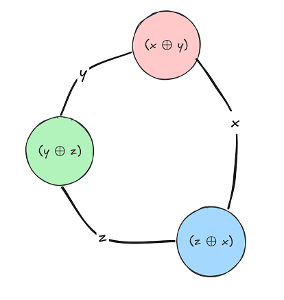
This exact limitation motivated the development of Rateless IBLTs, which eliminate the need to predict the required table size in advance.
Rateless IBLTs (R-IBLTs)
As we established, standard IBLTs have the flaw that they require prior knowledge of the approximate set difference size. Guess too large, and network bandwidth is wasted transmitting mostly empty cells. Guess too small, and peeling will fail to recover all differences, forcing the entire IBLT to be discarded while the peer rebuilds it with a larger number of cells.
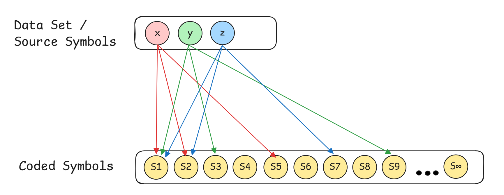
R-IBLTs remove this requirement by decoupling the data structure from a fixed-size table. Instead of mapping items into a predetermined M-cell table, an R-IBLT conceptually maps items onto an infinite sequence of cells, allowing those cells to be generated incrementally until peeling succeeds. This eliminates the need to estimate the set difference size in advance.
An R-IBLT cell differs slightly from a standard IBLT cell. For one the ValSum field disappears entirely since R-IBLTs are designed for set reconciliation, rather than key-value storage as there are no associated values to recover. The terminology also changes slightly. What a standard IBLT calls a cell, the R-IBLT paper refers to as a Coded Symbol, while the original inserted items are called Source Symbols.
SymbolSum - The ⊕ of all the source symbols mapped to this coded symbol by the generator functions (which we will discuss in detail shortly). This field serves the same role as the KeySum in a standard IBLT, but reflects the terminology used in the rateless version.
CheckSum - The ⊕ of all the hashes of all source symbols mapped to this coded symbol. This field serves the exact same purpose as with the regular IBLTs.
Count - A signed integer tracking the net number of source symbols currently mapped to this coded symbol. This field serves the exact same purpose as with the regular IBLTs.
During reconciliation, server A begins sending a stream of coded symbols to server B. Server B continuously attempts to peel the difference. If server B encounters a k-core deadlock, it does NOT fail, it simply asks server A for the next batch of coded symbols from the infinite sequence.
This continues until the collision graph breaks and all differences are resolved. There is no need to guess the size of the set difference in advance, and there is no wasted bandwidth sending empty cells. The R-IBLT being rateless can generate as many coded symbols as needed to successfully reconcile the sets.
Below we can see how a finite number source symbols are mapped to an infinite number of coded symbols, and that all source symbols map to 0th coded symbol. This is intentional because in R-IBLTs we know the peeling process is complete once we have fully peeled the 0th symbol, because all elements map to it by construction.
Majority of the work in the paper is to find a formula for the generator functions which yields a mapping probability, so that source symbols are not mapped to densely (or sparsely) to the infinite sequence of coded symbols.
Map too densely, and too many source symbols will collide within the same coded symbols, causing the Count of many cells to remain greater than one. Since peeling can only begin from pure coded symbols (cells with exactly 1 source symbol), excessive collisions can prevent the decoder from finding any starting points and the peeling process can not make progress.
Map too sparsely, and too many coded symbols will remain empty, meaning that the first O(|S|) coded symbols may not contain enough non-empty symbols to recover all source symbols. Since each pure coded symbol can recover at most one source symbol, insufficient non-empty symbols break the conditions required for successful decoding.
IBLT Prefix
To balance this mapping probability across an infinite sequence, an R-IBLT relies on evaluating prefixes of the sequence. If server A transmits a prefix of length L (say the first 100 coded symbols) and server B hits a deadlock, server A does not discard the data. It simply generates and transmits the next segment of the sequence (symbols L+1 through L+Δ). Server B appends these new symbols to its existing prefix and immediately resumes the peeling algorithm.
Because of this extensible prefix design, R-IBLTs size themselves to the actual set difference, d. You do not need to over-provision to guarantee pure cells. Mathematically, for any d > 0, on average, reconciling d-differences requires only the first 1.35d - 1.72d coded symbols in the sequence, which makes this method very efficient in terms of communication cost.
The overhead peaks at 1.72dl when d = 4, and stabilizes at 1.35dl as d increases in the low hundreds, where l is the length or number of bytes required to represent a source symbol. Computationally, R-IBLTs are also very efficient, requiring O(l log d) per set item (for encoding), and O(l log d) per set difference (for decoding).
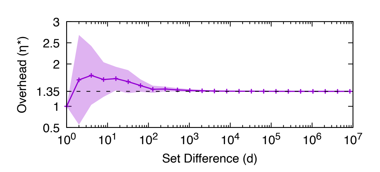
The protocol streams almost (more on this later) the minimum amount of symbols required to resolve the set difference. For R-IBLTs to work properly, they rely on 3 fundamental properties:
Decodability: The sequence guarantees that once a sufficient prefix length is reached (crossing the threshold bound relative to d), the stream will have produced enough pure symbols for the peeling algorithm to extract all missing items (with high probability).
Linearity: The commutative and associative properties of the ⊕ operator remain valid across the infinite sequence. Ci (A) ⊕ Ci (B) = Ci (A Δ B); meaning the ith symbol of server A ⊕ the ith symbol of server B will always equal the ith symbol of the set difference.
Universality: The decoding probability depends only on the magnitude of the set difference d, not the dataset itself, making the R-IBLT universally adaptable to any dataset without requiring parameterization (or prior heuristics).
Mapping Probability
To solve the density vs sparsity problem mentioned above, we can no longer rely on a set number of hash functions (like k=3) for every item. If every source symbol mapped to the exact same number of coded symbols (its degree), the resulting graph would be too uniform, thereby heavily increasing the likelihood of k-core deadlocks / cyclic loops. Instead, the degree of each source symbol is chosen dynamically from a carefully weighted probability distribution.
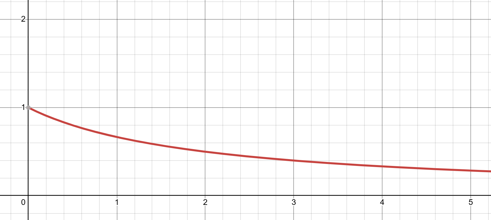
Let p(i) be the probability distribution function or as referred in the paper as the mapping probability, defining the likelihood that a random source symbol maps to the ith coded symbol.
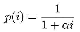
The authors chose p(i) so that it is inversely proportional to i (creating a heavy-tailed, left-sided distribution) to balance 2 competing (low vs high degrees) needs of the peeling algorithm:
Low Degrees (kick-starting an avalanche): The algorithm relies on pure cells (degree = 1) to begin decoding. A left-sided, inversely proportional shape ensures the vast majority of source symbols are assigned very low degrees (1 or 2), thereby ensuring a large initial pool of pure cells to start a "chain reaction" of peeling.
High Degrees (preventing isolation): If all items had low degrees, some items might never be mapped into the sequence at all, remaining permanently isolated. The heavy-tail ensures a small but critical number of items get very high degrees. These act as massive interconnected hubs, guaranteeing (again with high probability) every source symbol is tied into the graph at least once.
To select a degree at runtime, the authors rely on the cumulative distribution function (CDF), denoted as C(x). The CDF gives us the probability that a random variable X will take a value less than or equal to x:
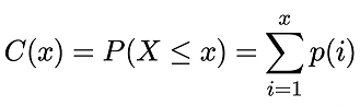
From a pure theoretical prespective, to assign a degree to a source symbol, you would generate a random floating-point number r ∈ [0,1), and use C-1(r) (the inverse CDF) to find the corresponding degree.
The authors select the constant α = 0.5. The reason for this very specific choice is purely for computational efficiency. Computing the inverse CDF when α = 0.5 simplifies the equation so that it only requires computing square roots. If any other value for α were chosen, C-1(r) would involve raising (1 − r) to non-integer powers, which is computationally more expensive.

Recall on the previous section, we said:
The protocol streams almost the minimum amount of symbols required to resolve the set difference
The reason why it is "almost" is because the authors picked α = 0.5 (again for computational efficiency), but this comes at a cost of slightly increasing the number of coded symbols that need to be streamed. The authors note that the optimal value is actually α = 0.64, which would reduce the number of coded symbols sent from 1.35d to 1.31d (a decrease of 3%), but this would require computing (1 − r)0.63, which is more expensive than computing sqrt(1 − r).
Generator Function
Now that we understand the heavy-tailed mapping probability, we need to translate this into code. To map a source symbol onto the infinite sequence of coded symbols, we need a deterministic "schedule" of indices.
The paper defines the generator function to find the next index using this specific inverse CDF formula:

If we compute this by first generating r say using Random.Shared.NextDouble() and raising (1 - r) to a fractional power via Math.Pow(), the CPU overhead would be significant. To make this efficient, we rely on a substitution trick. If we use a 64-bit pseudo-random number generator (PRNG), our generated state X falls uniformly in the range [0, 264).
We can express r as:
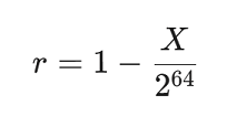
Or in terms of (1 - r):
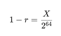
We can now substitute this back into the expensive part of the generator function:

To prevent a divide-by-zero error when the PRNG yields exactly 0, we simply define X as:
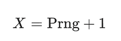
Because 232 = 4294967296, we reduce the complex inverse CDF random sample calculation to the following form:
double inverseCdfSample = (4294967296.0 / Math.Sqrt(Prng + 1.0)) - 1.0After having obtained the inverse CDF sample, we calculate the jump (the distance to the next coded symbol in the infinite sequence):
double jump = Math.Ceiling((LastIndex + 1.5) * inverseCdfSample);

long nextIndex = Math.Max(1L, jump >= int.MaxValue ? int.MaxValue : (long)jump);

LastIndex += nextIndex;
To understand why it is calculated this way, we have to look at the 3 mechanisms at play:
Progressive Sparsity: (LastIndex + 1.5) * inverseCdfSample
Notice that the random sample inverseCdfSample is multiplied by the LastIndex. This means that the further down the sequence we go, the larger the jumps become.
When a source symbol is just starting its sequence (LastIndex = 0), the multiplier is small (1.5), meaning the first few coded symbols it maps to will be clustered tightly near the beginning of the sequence. This guarantees a high density of items in the early cells, providing the pure cells needed to kick-start the peeling avalanche.
However, as LastIndex grows, multiplying it by the random sample produces exponentially larger gaps. This ensures that deep into the infinite sequence, the mapping becomes very sparse, preventing the k-core deadlocks associated with uniform hashing.
Monotonic Progress: Math.Max(1L, ...)
Because inverseCdfSample can theoretically evaluate to 0 (when Prng hits its absolute maximum), the resulting jump could also be 0. In that case the generator would yield the exact same index twice in a row, ⊕'ing the source symbol against the same coded symbol twice.
Because x ⊕ x = 0, the item would self-cancel from that cell!
Taking Math.Max(1L, ...) strictly enforces monotonic progress, ensuring the symbol always advances by at least one cell.
Overflow Protection: >= int.MaxValue
Because inverseCdfSample can be up to 4.2 billion (since Prng can be up to uint.MaxValue), and it is being multiplied by a growing LastIndex, the jump grows very fast and could exceed long.MaxValue in just 2 or 3 iterations, causing an integer overflow that wraps around into negative numbers.
We clamp the maximum jump to int.MaxValue, so we are safely within bounds.
In the context of an actual implementation, any index beyond the size of the allocated array is naturally skipped anyway (because arrays in .NET have a maximum length of int.MaxValue). Clamping it simply keeps the math safe without affecting the logical sparsity of the R-IBLT.
Putting it all together, the generator function (refered to as RandomMapping) could be implemented as follows:
internal struct RandomMapping(ulong hash, long startIndex = 0)
{
    public ulong Prng = hash;
    public long LastIndex = startIndex;

    [MethodImpl(MethodImplOptions.AggressiveInlining)]
    public long NextIndex()
    {
        // This is the deterministic PRNG update step taken from
        // the paper, which provides high quality randomness,
        // assuming the multiplier is co-prime to 2^64.
        Prng *= 0xda942042e4dd58b5UL;

        double inverseCdfSample = (4294967296.0 / Math.Sqrt(Prng + 1.0)) - 1.0;
        double jump = Math.Ceiling((LastIndex + 1.5) * inverseCdfSample);

        long nextIndex = Math.Max(1L, jump >= int.MaxValue ? int.MaxValue : (long)jump);

        LastIndex += nextIndex;

        return LastIndex;
    }
}
Lets compare this version against a naive approach where we literally compute r and use Math.Pow(1.0 - r, -0.5) to evaluate the fractional power:
internal struct NaiveRandomMapping(ulong hash, long startIndex = 0)
{
    public ulong Prng = hash;
    public long LastIndex = startIndex;

    [MethodImpl(MethodImplOptions.AggressiveInlining)]
    public long NextIndex()
    {
        Prng *= 0xda942042e4dd58b5UL;

        double r = 1.0 - (Prng / 18446744073709551616.0); // 1 - (Prng / 2^64)

        double inverseCdfSample = Math.Pow(1.0 - r, -0.5) - 1.0;
        double jump = Math.Ceiling((LastIndex + 1.5) * inverseCdfSample);
        long nextIndex = Math.Max(1L, jump >= int.MaxValue ? int.MaxValue : (long)jump);

        LastIndex += nextIndex;

        return LastIndex;
    }
}
The benchmark below executes both version's NextIndex() for a total of 10,000 times. The results show the optimized version is ~7x faster! This is a substantial result considering this operation is executed for every single jump, of every single source symbol, during both the encoding and peeling phases. This allows the CPU to spend its time doing math for resolving set differences, rather than doing unnecessary calculations for jumps, allowing the R-IBLT to run entirely allocation-free and single-digit nanosecond fast ~4.6 [ns] / op.

Mapping Heap
To generate the R-IBLT, the encoder must evaluate the rateless stream chronologically (from index 0 upwards to infinity). Because every source symbol follows its own deterministic sequence of jumps, we need a way to know which source symbol maps to the current coded symbol, without having to simulate the entire infinite sequence for every item.
This is a classic scheduling problem. To solve it, the authors use a heap! In our code its encapsulated in a MappingHeap which is a high-perf, min-heap (priority queue, but faster) custom-built for the R-IBLT encoder. Elements inside the heap are ordered by their target CodedIndex. The root element always represents the symbol scheduled for the lowest (earliest) future index.
This allows the CodingWindow to act as a self-moving conveyor belt. It efficiently evaluates the rateless stream in O(log N) time, applying any scheduled source symbols into the provided coded symbol and advancing the sequence.
Because the sequence generation sits on the absolute hottest path of the reconciliation engine, we avoid using a standard PriorityQueue which would introduce substancial overhead. Instead we build an optimized version of the heap for this purpose and employ several optimizations to maximize throughput but also reduce allocations.
In-Place Root Mutation and Ref-Returns:
Whenever a source symbol is applied to the current cell, we need to calculate its next jump and re-queue it. Dequeueing and re-enqueueing structs causes memory copying. Instead, MappingHeap exposes the root element by reference:
[MethodImpl(MethodImplOptions.AggressiveInlining)]
public ref SymbolMapping Peek() => ref MemoryMarshal.GetReference(CollectionsMarshal.AsSpan(_mappings));
Adapting to the Heavy-Tailed Distribution (Floyd's Optimization):
Once the caller mutates the root (by updating its CodedIndex to the next jump), they must call UpdateRoot() to rebalance the heap. Because the R-IBLT uses a heavy-tailed distribution, most source symbols will map to the first few coded symbols, and only a few will map to the later coded symbols.
Profiling shows that on almost every jump, the root will be replaced with a child, and then that child will be replaced with its child, moving the root deep down the heap. Instead of performing 3-way swaps at every level, we implement Floyd's Optimization.
We save a copy of the mutated root before we start shifting things up, otherwise we will overwrite it on the very first iteration. Than we sift down to the bottom of the heap, blindly pulling up the minimum child at each step to create a "hole".
while (current < limit)
{
    int leftChildIndex = (current * 2) + 1;
    int rightChildIndex = leftChildIndex + 1;

    ref SymbolMapping left = ref Unsafe.Add(ref ptr, leftChildIndex);
    ref SymbolMapping right = ref Unsafe.Add(ref ptr, rightChildIndex);

    // Find the smallest child
    int minChildIndex = left.CodedIndex <= right.CodedIndex ? leftChildIndex : rightChildIndex;

    // Pull the smallest child up to fill the current hole
    Unsafe.Add(ref ptr, current) = Unsafe.Add(ref ptr, minChildIndex);

    current = minChildIndex;
}
After sifting the hole down to the leaf level, we execute a short sift-up phase to place the saved root element into its final position. This dramatically minimizes the number of swaps and copies during the sequence generation.
int half = count >> 1; // Essentially count / 2, which is the first index that is guaranteed to have at least one child.

if (current < half)
{
    int leftChildIndex = (current << 1) + 1;
    Unsafe.Add(ref ptr, current) = Unsafe.Add(ref ptr, leftChildIndex);
    current = leftChildIndex;
}

// We sift up to final resting place, which means we are done with the "hole"
// and we can place the saved root element into its final position.
while (current > 0)
{
    int parentIndex = (current - 1) / 2;
    ref SymbolMapping parent = ref Unsafe.Add(ref ptr, parentIndex);

    if (parent.CodedIndex <= newCodedIndex)
    {
        break;
    }

    Unsafe.Add(ref ptr, current) = parent;
    current = parentIndex;
}

// Now we just drop the saved root into its final resting place.
Unsafe.Add(ref ptr, current) = rootMapping;
The CodingWindow than evaluates the infinite R-IBLT sequence at the exact NextIndex, applying any scheduled source symbols into the provided coded symbol and advancing the sequence i.e. NextIndex.
The actual code has extra instrumentation which is stripped off below.
internal enum SymbolOperation
{
    Add = 1,
    Remove = -1
}

internal class CodingWindow
{
    private readonly MappingHeap _queue = new();
    private readonly List<HashedSymbol> _symbols = [];
    private readonly List<RandomMapping> _mappings = [];

    ...

    public CodedSymbol ApplySymbol(CodedSymbol symbol, SymbolOperation operation)
    {
        if (_queue.Count == 0)
        {
            NextIndex++;
            return symbol;
        }

        var symbolsSpan = CollectionsMarshal.AsSpan(_symbols);
        var mappingsSpan = CollectionsMarshal.AsSpan(_mappings);

        // We peek at the top to see which source symbol
        // will be mapped to this coded symbol.
        ref var root = ref _queue.Peek();

        while (root.CodedIndex == NextIndex)
        {
            var index = root.SourceIndex;

            // And proceed to 'apply' the source symbol (contained within hashed symbol) into the coded symbol.
            // This will perform the IBLT math: XOR'ing the source symbol's ID, and Hash into the cell,
            // and adjusting the cell's count (+1 for Add, -1 for Remove)
            symbol.Apply(symbolsSpan[index], operation);

            // Push this symbol's *next* mapping into the future.
            root.CodedIndex = mappingsSpan[index].NextIndex();

            // UpdateRoot will sift this element down and bring the next smallest item to index 0.
            // On the next loop iteration, 'root.CodedIndex' automatically evaluates the *new* minimum element!
            _queue.UpdateRoot();
        }

        // The current cell is now fully constructed,
        // so we advance the sequence to the next timestep.
        NextIndex++;

        return symbol;
    }
}
Why a heap?
Regardless of the code optimizations, the choice to use a min-heap over a simple list scan fundamentally comes down to algorithmic time complexity and the sparse nature of the R-IBLT sequence. If we were to use a naive scanning approach, the CodingWindow would have to iterate through every single source symbol in the cache for every single coded symbol it generates to see if it belongs there.
If a node has 1,000,000 source symbols, and it needs to generate 10,000 coded symbols to resolve a difference, a full scan would require:
1,000,000 [source symbols] × 10,000 [coded symbols] = 10,000,000,000 evalsNeedless to say that this O(N) per-cell time complexity scales terribly, but it is especially devastating for R-IBLTs because of progressive sparsity. As we discussed earlier, the gaps between jumps become exponentially larger the further down the sequence we go.
Deep in the sequence, a coded symbol might only have 1 or 2 source symbols mapped to it, or it might be completely empty. A scanning approach would force evaluation of all 1,000,000 items just to find the 2 items that actually land on that specific cell, thereby wasting millions of cycles doing nothing.
By using a min-heap such as our MappingHeap which is ordered by the target CodedIndex, we eliminate all that waste work. The root of the heap explicitly tells us exactly which symbol is up next. If the root's scheduled index is further in the future than our current cell, we instantly know that no symbols map to the current cell. We just advance the sequence without checking the rest of the dataset. When we do process a symbol, removing it and re-inserting its next jump back into the heap only takes O(log N) operations.
The heap allows the encoder to leapfrog over the massive empty gaps in the heavy-tailed distribution thereby processing the rateless stream with peak efficiency (to my best knowledge).
Mutation Symbol
To maximize throughput, the MutationSymbol (the fundamental unit of exchange) which wrapps a 16-byte Guid is heavily optimized as it is in one of the hottest paths: ⊕'ing & hashing.
For the ⊕ operation, we completely bypass byte-level iteration. When SIMD hardware acceleration is available, we load the ID directly into a Vector128 register (because a Guid is exactly 128 bits), thereby performing a 128-bit ⊕ as a single vector operation.
internal readonly record struct MutationSymbol(Guid Id)
{
    [MethodImpl(MethodImplOptions.AggressiveInlining)]
    public MutationSymbol Xor(MutationSymbol other) =>
        new(Vector128.IsHardwareAccelerated ? SimdXor(Id, other.Id) : ScalarXor(Id, other.Id));

    [MethodImpl(MethodImplOptions.AggressiveInlining)]
    public static Guid SimdXor(Guid id, Guid otherId)
    {
        Guid result = default;

        var idVec = Vector128.LoadUnsafe(ref Unsafe.As<Guid, byte>(ref id));
        var otherIdVec = Vector128.LoadUnsafe(ref Unsafe.As<Guid, byte>(ref otherId));
        var resultVec = idVec ^ otherIdVec;

        resultVec.StoreUnsafe(ref Unsafe.As<Guid, byte>(ref result));

        return result;
    }

    ...
}
Majority of computers nowdays support 128-bit SIMD instructions, but just in case not, we fallback to doing word-level parallelism since we know the ID will be fixed at 128 bits. We first point to the very beginning of the Guid's as raw bytes, and read them as unaligned reads (this way we allow the runtime to generate the appropriate code regardless of the underlying CPU alignment requirements) to process the 128 bits as 2 x 64-bit integer operations. This way we reduce the work from 16 → 2 ⊕ operations, which is a substantial speedup.
internal readonly record struct MutationSymbol(Guid Id)
{
    ...

    [MethodImpl(MethodImplOptions.AggressiveInlining)]
    public static Guid ScalarXor(Guid id, Guid otherId)
    {
        Guid result = default;

        const int WordLength = 8;

        ref byte idBytes = ref Unsafe.As<Guid, byte>(ref id);
        ref byte otherBytes = ref Unsafe.As<Guid, byte>(ref otherId);
        ref byte resultBytes = ref Unsafe.As<Guid, byte>(ref result);

        ulong low = Unsafe.ReadUnaligned<ulong>(ref idBytes) ^ Unsafe.ReadUnaligned<ulong>(ref otherBytes);
        ulong high = Unsafe.ReadUnaligned<ulong>(ref Unsafe.Add(ref idBytes, WordLength)) ^ Unsafe.ReadUnaligned<ulong>(ref Unsafe.Add(ref otherBytes, WordLength));

        Unsafe.WriteUnaligned(ref resultBytes, low);
        Unsafe.WriteUnaligned(ref Unsafe.Add(ref resultBytes, WordLength), high);

        return result;
    }
}
The same principle applies to hashing. Since the ID is fixed at 128 bits, there is no need to process it as a sequence of individual bytes. We again reinterpret the Guid as raw memory and load it as 2 × 64-bit words using unaligned reads.
We then mix the 2 words together using the golden ratio's 64-bit fixed-point representation of the fractional part. We this specific value for its useful bit-mixing properties, as it is a highly irrational number.
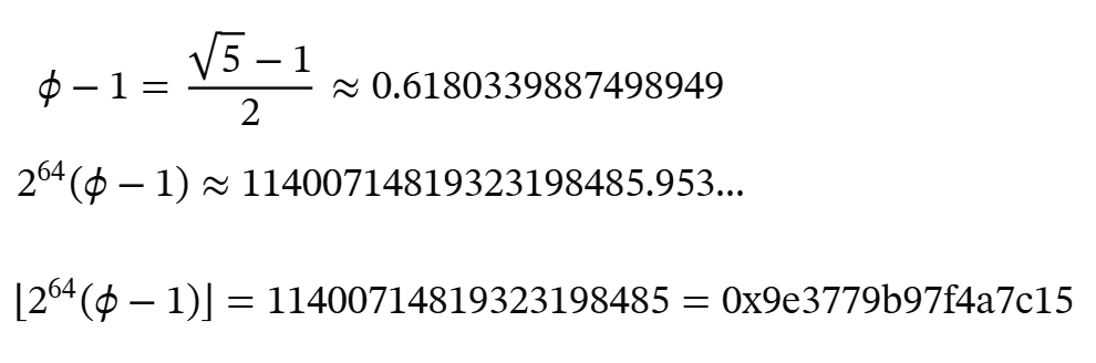
A useful property of the golden ratio is that its successive multiples produce a well-distributed sequence of fractional values. For an irrational number c, consider the following:
frac_part = (n x c) % 1Where c is the constant being tested. With c = Φ - 1, the resulting values are spread very evenly across [0,1). Other constants such as π or e also produce non-repeating sequences, but the golden ratio gives particularly good distribution with minimal clustering, because it is one of the hardest to approximate with fractions. The plot below illustrates this behavior for the golden ratio.
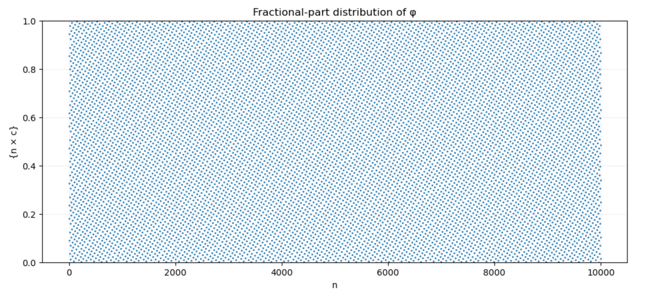
The purpose here is to mix the 2 halves of the ID so that correlations between them are less likely to carry into the resulting 64-bit hash value. A final right-shift further mixes the upper and lower portions of that 64-bit value, helping to spread the input's bit information throughout the hash.
[MethodImpl(MethodImplOptions.AggressiveInlining)]
public ulong GetHash()
{
    Guid id = Id;

    const int WordLength = 8;

    ref byte idBytes = ref Unsafe.As<Guid, byte>(ref id);

    ulong low = Unsafe.ReadUnaligned<ulong>(ref idBytes);
    ulong high = Unsafe.ReadUnaligned<ulong>(ref Unsafe.Add(ref idBytes, WordLength));

    const ulong GoldenRatioFraction = 0x9e3779b97f4a7c15UL;

    ulong mixedHash = low ^ (high + GoldenRatioFraction);
    mixedHash ^= mixedHash >> 32;

    return mixedHash == 0 ? 1 : mixedHash;
}
This gives us a compact 64-bit hash from the 128-bit ID using only: 2 memory reads, 1 addition, 1 XOR, and 1 right-shift.
Dont confuse the 64-bit hash (as
GetHash()returns aulong) with the input itself (theGuid) which is 128 bits.
The final mixedHash == 0 ? 1 : mixedHash; guard is intentional, as GetHash() is used as the seed for the generator function RandomMapping, whose PRNG state must never start at zero (since a zero state would cause it to remain permanently stuck). By replacing 0 → 1, we preserve the deterministic mapping while eliminating that problematic state.
Profiler Results
To validate whether these low-level heap optimizations were actually necessary, I built a custom profiling suite to trace the exact behavior of the encoder. The cache was loaded with 1,000,000 items and generated coded symbols in batches to see exactly where the CPU was spending its time. The profiler outputs reveal exactly why the MappingHeap is so important.
==================================================
                 RIBLT PROFILER REPORT
==================================================

--------------- HIGH-LEVEL METRICS ---------------
Symbols Produced:       1,000,000
Empty Symbols:          37,659
Non-Empty Symbols:      962,341

--------------- WORKLOAD PERFORMANCE ---------------
Total Loop Iterations:  26,730,889
Max Iterations/Symbol:  1,000,000
Avg Iterations/Symbol:  26.73

--------------- ALGORITHM BEHAVIOR ---------------
UpdateRoot Calls:      26,730,889
UpdateRoot Rate:       100.00%
The takeaway from the profiling data is the Algorithm Behavior section. Across all 26.73 million loop iterations, the UpdateRoot() method was called exactly 26.73 million times (100% rate). This shows that updating the root element is the absolute hot spot of the entire algorithm (at least on the encoder/generation side). Every single time the CodingWindow evaluates a source symbol, it must compute its NextIndex and re-queue it.
If we were executing standard dequeue/enqueue operations or performing 3-way swaps up and down the heap on every single iteration, the overhead would have been substantially larger. Employing the optimizations is what allows the encoder to churn through millions of iterations in milliseconds.
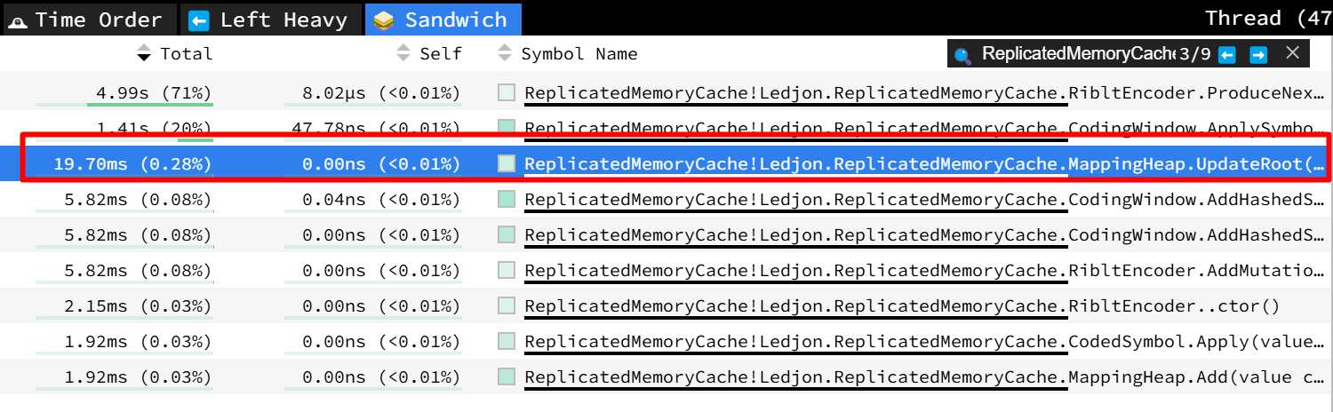
Similar observation can be made by loading a profiling session into speedscope. Note that I filtered the trace strictly to the library's namespace to isolate the engine from the benchmarking code overhead. In speedscope, total time measures time spent in a method including its child calls, while self time measures time spent exclusively within that method.
The sandwich view confirms the encoder spends its time where it should:
- ProduceNextSymbol: 4.99s (71%) orchestrating sequence generation.
- ApplySymbol: 1.41s (20%) performing the ⊕ and hashing math.
- ReplaceRoot: 19.78ms (0.28%) maintaining the heap.
Despite executing on 100% of iterations, the heap maintenance accounts for 0.28% of execution time. It may not be obvious why its self time is effectively 0.00 [ms] (<0.01%), but this is due to aggressive inlining. The JIT dissolves the method boundaries entirely. When the profiler pauses the CPU to take a snapshot, it almost never catches the CPU executing the "wrapper" code of UpdateRoot().
Distribution Analysis
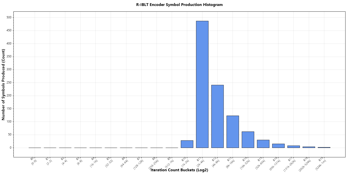
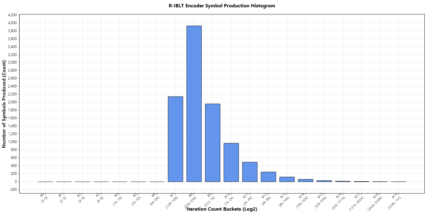
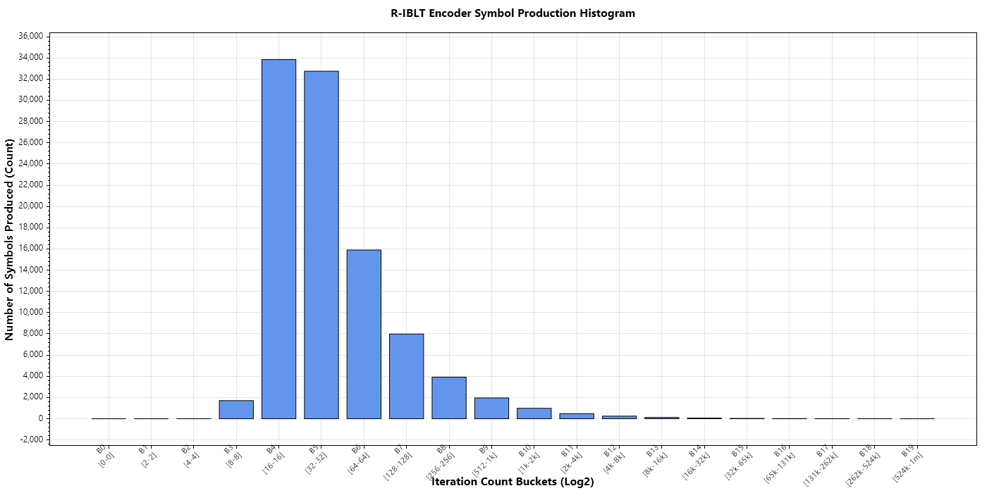
To see exactly how the algorithmic workload shifts over time, we can plot the iteration counts of the profiling session into logarithmic buckets. Below is a visual progression (via histograms) of the encoder as it generates from 1 to 1,000,000 coded symbols.
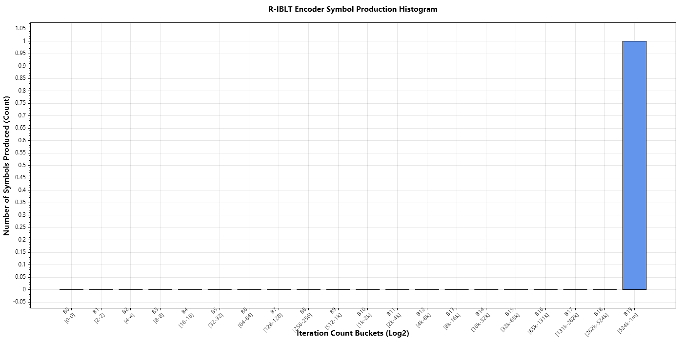
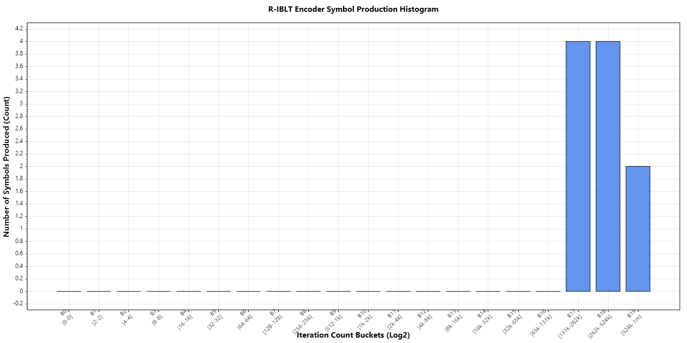
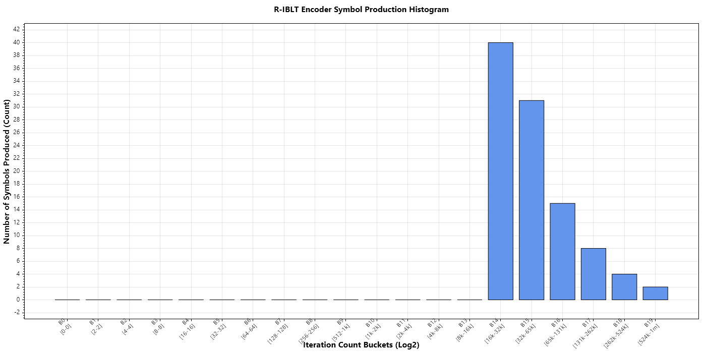
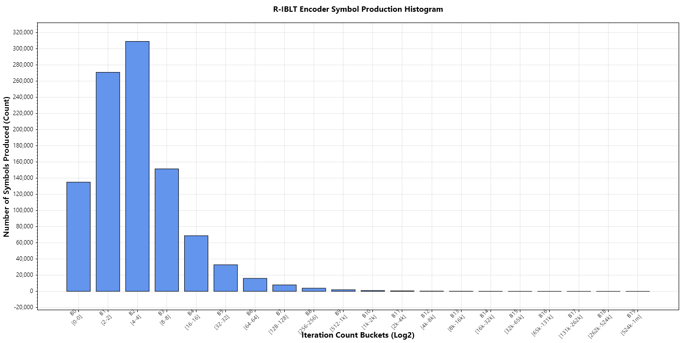
Notice the right → left shift as the number of produced coded symbols increases. When producing the very first symbol (first picture), the histogram is entirely concentrated in Bucket 19. Because the encoder is starting from scratch, every single one of the 1,000,000 source symbols in the cache must be hashed and sifted through the heap at least once to find its starting index.
As we generate 1,000 to 10,000 symbols, the distribution spreads more across the middle buckets. The heap is actively sorting the future jump indices of the symbols. By the time we reach the 1,000,000 symbol mark, the vast majority of the work has shifted to buckets [0, 4] (0-31 iterations per symbol).
This leftward shift shows the efficiency of the MappingHeap. As the CodingWindow advances, the sequence becomes progressively sparser. Source symbols that have exhausted their pseudo-random jumps are naturally left behind by the root of the heap. Instead of scanning all 1,000,000 items to assemble the final coded symbols, the encoder leapfrogs over the empty space, and picks out only the handful of items that actually belong in that specific cell.
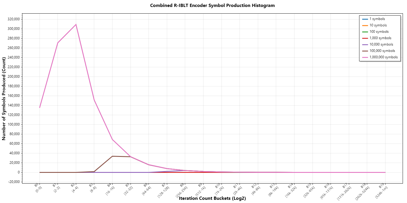
For reference here is a combined view of all cases expressed in a line chart.
Encoder Benchmarks
To measure the throughput and verify the zero-alloc design, we run the encoder through a suite of benchmarks to see the computational cost of resolving set differences of varying sizes across different cache sizes. The suite is divided into 2 parts: measuring the cold start (the very first symbol), and measuring the sustained generation of coded symbols.
Cold Start Penalty

The benchmark results for producing the first symbol mirror the right-heavy "Bucket 19" from the first histogram. Generating the first symbol requires O(N) work, where N is the size of the cache. Every single item (these are not the contents, but rather mutation ids) in the cache must be: hashed, evaluated, and sifted through the heap at least once to determine its starting position on the sequence. For 1,000,000 items, this initial full cache scan takes about ~106 [ms].
Sustained Generation Cost
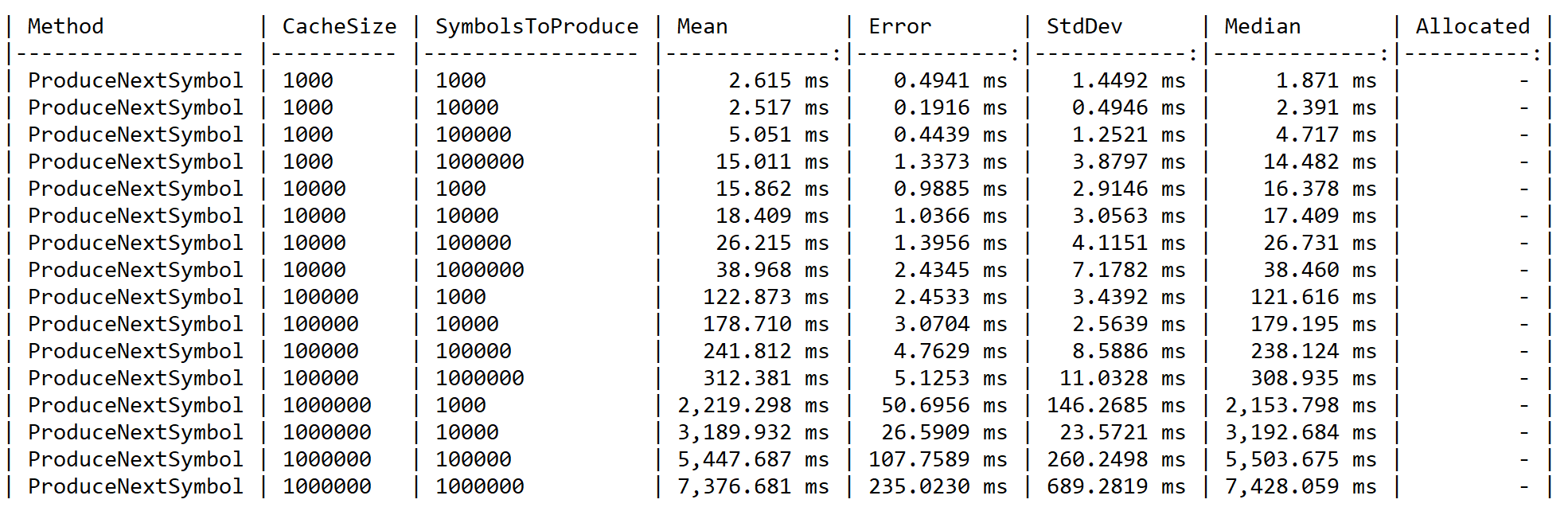
Lets put focus on how the execution time scales across 2 dimensions:
- The size of the data/cache (N).
- The length of the generated sequence / symbols to produce (K).
Cache Size Cost
The results show that the overall execution time is dominated by the number of items in the cache, not the number of symbols being generated. If we look at a fixed output of 1,000 symbols, the cost scales directly with the cache size:
- N = 1,000: ~2.61 ms
- N = 10,000: ~15.86 ms
- N = 100,000: ~122.87 ms
- N = 1,000,000: ~2,219.29 ms
As the cache grows, the initial O(N) cold start penalty increases. The encoder has a much larger working set to evaluate, memory locality (L1/L2 cache misses) becomes a factor, and the O(log N) heap grows deeper. The vast majority of the computational effort is spent processing this massive initial wave of symbols all fighting for placement in the earliest windows.
Sequence Length Cost
However, the true power of the algorithm is revealed when we look at the horizontal scaling. Regardless of how large N is, the cost of producing more symbols (K) remains astonishingly low. Looking at the execution times across the N = 1,000,000 rows in the benchmark results:
- K = 1,000: ~2.22 secs
- K = 10,000: ~3.19 secs (10x symbols → 1.4x time)
- K = 100,000: ~5.45 secs (100x symbols → 2.45x time)
- K = 1,000,000: ~7.38 secs (1,000x symbols → 3.3x time)
If the computational cost scaled as O(K), generating 1,000,000 symbols would have taken over 2,200 secs (36.6 mins). Instead, producing 1,000x more data takes 3.3x the original duration. We see the same sub-linear amortization for N = 100,000 where a 1,000x symbols increase (K = 1,000 - 1,000,000) only yields a 2.55x time increase (122 → 312 [ms]).
The encoder essentially front-loads its work based on the cache size. Once that initial wave is processed, the heavy-tailed distribution takes over, causing the marginal cost per generated symbol to plummet towards 0. This can be explained by the mechanics of the R-IBLT generation loop as follows:
Front-Loaded Workload: The N-dimension drives the initial processing time. Every item in the cache must be evaluated, absorbing almost the entire computational penalty in the earliest stages of the symbol generations.
Rapid Jump Exhaustions: As the window advances along the K-dimension, the workload collapses. Because the degree distribution is heavily skewed toward small values, most source symbols only map to a few early coded symbols before exhausting their jump sequence (recall that the jumps becomes exponentially larger).
Heap Attrition: As symbols exhaust their jumps, they are permanently discarded. The MappingHeap shrinks drastically, requiring less and less operations so this marginal cost per generated symbol plummets towards 0.
R-IBLT Sketch
While the mathematical foundation of the R-IBLT is highly efficient for infinite stream generation, dynamically computing that stream on-demand introduces a performance penalty upon large-sized caches, majority of it belonging to the mapping of source symbols to the very first coded symbol. This is the cold start problem we talked about earlier. To bypass this problem we built a sketch for the R-IBLT.
The sketch acts as a pre-computed prefix buffer that continuously materializes the first S coded symbols (8,192 by default) of the rateless stream. By maintaining this buffer and updating it alongside cache operations, the sketch completely eliminates the need for constant encoder hydration when reconciling d set differences (given d <= S).
The sketch is implemented as a fixed-size buffer of CodedSymbol's. Recall that R-IBLTs possess the linearity property, this allows mutations (IDs of changes made to cache items) to be mapped directly across the buffer using pseudo-random indices derived from each symbol's hash. To prevent race conditions during concurrent updates, the buffer makes use of a striped-locking pattern to isolate cell mutations without having to serialize access across the entire buffer.
internal class RibltSketch
{
    private const int LockCount = 64; // MUST be a power of 2 for bitwise masking.
    private const int LockMask = LockCount - 1;

    private readonly CodedSymbol[] _buffer;
    private readonly Lock[] _lockStrip = [.. Enumerable.Range(0, LockCount).Select(_ => new Lock())];

    ...

    public void ApplyMutation(MutationSymbol symbol, SymbolOperation operation)
    {
        var hashedSymbol = new HashedSymbol(symbol, symbol.GetHash());
        var mapping = new RandomMapping(hashedSymbol.Hash, 0);

        while (mapping.LastIndex < _buffer.Length)
        {
            int index = (int)mapping.LastIndex;
            var lockObj = _lockStrip[index & LockMask];

            lock (lockObj)
            {
                // We lock here to prevent lost updates during the RMW cycle.
                // Applying a symbol involves non-atomic XOR and addition
                // operations across 32 bytes (CodedSymbol size). If two separate
                // cache updates PRNG-collide on this exact cell simultaneously
                // without a lock, their XORs would interleave and
                // corrupt the cell's math.

                _buffer[index].Apply(hashedSymbol, operation);
            }

            mapping.NextIndex();
        }
    }

    public int ReadSlice(int offset, Span<CodedSymbol> destination)
    {
        var resultCount = Math.Min(destination.Length, _buffer.Length - offset);
        if (resultCount <= 0)
        {
            return 0;
        }

        for (int i = 0; i < resultCount; i++)
        {
            int index = offset + i;
            var lockObj = _lockStrip[index & LockMask];

            lock (lockObj)
            {
                // We must lock the read to prevent a torn-read since
                // CodedSymbol is 32 bytes (CPU cant copy it atomically).
                // If we dont lock, a concurrent write could alter the cell mid-copy,
                // resulting in a mathematically corrupted symbol.
                // This could happen when a reconcilliation/gossip thread tries to read a slice,
                // at the exact same time a cache thread is updating that same cell.
                // Since we lock, we can copy the 32-byte struct into the caller's span.
                // This guarantees the caller gets a valid snapshot of the cell,
                // without allocating on the heap.

                destination[i] = _buffer[index];
            }
        }

        return resultCount;
    }
}
When a reconciliation round requires pulling more data than the sketch provides, we transition from the sketch to the dynamic encoder using AddMutationAtOffset(symbol, offset). Rather than re-evaluating the sequence from the beginning, we fast-forward the CodingWindow. The encoder and decoder are symmetric as in: both simply feed their offset to AddHashedSymbolAtOffset(symbol, offset), which handles the PRNG fast-forward and repositions NextIndex to the given offset.
This is not part of R-IBLTs themselves, rather an extra optimization to avoid the cold start problem.
internal class RibltEncoder
{
    private readonly CodingWindow _window = new();

    ...

    public void AddMutationAtOffset(MutationSymbol symbol, long offset)
        => _window.AddHashedSymbolAtOffset(
            new HashedSymbol(symbol, symbol.GetHash()), offset);

    ...
}

internal class RibltDecoder
{
    private readonly CodingWindow _remote = new();

    ...

     public void AddMutationAtOffset(MutationSymbol symbol, long offset)
        => _current.AddHashedSymbolAtOffset(
            new HashedSymbol(symbol, symbol.GetHash()), offset);

    ...
}

internal class CodingWindow
{
    ...

    public void AddHashedSymbolAtOffset(HashedSymbol symbol, long offset)
    {
        var mapping = new RandomMapping(symbol.Hash, 0);

        // Fast-forward this symbol until it reaches the target offset.
        // We skip all intermediate cells because they are not needed
        // when reconstructing window state from an offset.
        // The point is to avoid the min-heap operations,
        // since we are not actually evaluating the intermediate cells.

        while (mapping.LastIndex < offset)
        {
            mapping.NextIndex();
        }

        // We also rewind NextIndex to 'offset' otherwise the window
        // will evaluate 'offset' number of empty cells before it
        // starts producing (or subtracting) anything meaningful.

        NextIndex = offset;

        AddHashedSymbol(symbol, mapping);
    }

    public void AddHashedSymbol(HashedSymbol symbol, RandomMapping mapping)
    {
        _symbols.Add(symbol);
        _mappings.Add(mapping);
        _queue.Add(new SymbolMapping
        {
            SourceIndex = _symbols.Count - 1,
            CodedIndex = mapping.LastIndex
        });
    }

    ...
}
The benchmark results for the sketch's read performance against the encoder producing the same-sized prefix highlights the advantage of the O(1) read access. Regardless of the underlying cache size the execution profile remains completely flat, with sketch read times stabilizing at ~150 [µs]. Ultimately, the O(1) extraction time makes the sketch highly effective for fast-path synchronization, allowing for rapid resolving of reasonably large set differences, without paying the computational cost of generating a rateless stream from zero.

The difference in memory footprint comes from how and when the underlying data structures are created. In the benchmark, the sketch and its buffer are instantiated once during the GlobalSetup phase. The measured Sketch_ReadPrefix() method directly copies the 32-byte structs from the buffer into destination span. Because no new objects are created during the read operation, it completes without doing any heap allocations.
In contrast, a new encoder must be instantiated for every benchmark iteration, because its internal state mutates as it generates the rateless stream. When loading up to 1,000,000 mutations, the encoder's internal array-baked collections (which track symbols, PRNG mappings, and the heap) must resize to accommodate the data. Each resize operation allocates a new, larger backing array and discards the previous one. At larger cache sizes, this continuous re-allocation/copying creates the memory pressure responsible for the observed Gen2 collections.
This looks unfair at first, but its actually not! This is more realistic since an encoder would be created per-reconcilliation round between 2 peers, whereas the sketch would stay the same for every round.
Why a sketch?
If you were reading carefully, you would notice that due to the linearity property of R-IBLTs, any prefix of a generated rateless stream is conceptually a sketch itself. If the architecture relied on a single centralized leader, that leader could generate this prefix and stream it to all replica nodes, effectively acting as a universal sketch for the entire cluster.
However, relying on a single node introduces a bottleneck. If the leader fails, synchronization halts. We are aiming for a decentralized, gossip-driven replication engine where nodes communicate randomly with each other.
In a pure peer-to-peer (P2P) model, any node can initiate a reconciliation round with any other random peer, at any given moment. Because these interactions are not coordinated, forcing the system to generate that prefix on-demand for every single gossip round would impact performance negatively.
By having every node continuously maintain its own explicitly materialized sketch in realtime, prefix exchanges across arbitrary P2P pairings enable convergence without bottlenecking on a leader, or paying the computational tax of re-encoding i.e. the cold start problem.
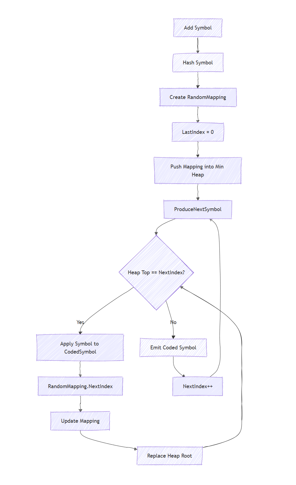
As we come to an end regarding the R-IBLT encoder, the diagram below gives an overview of how it handles the insertions of source symbols, and the production of coded sysmbols.
R-IBLT Decoder
Definitions
- LocalWindow: A list of cache items discovered the local node has, but the remote node is missing.
- RemoteWindow: A list of cache items discovered the remote node has, but the local node is missing.
- LocalDiscoveries: A list of coded symbols received from the remote stream, mutated in-place over time.
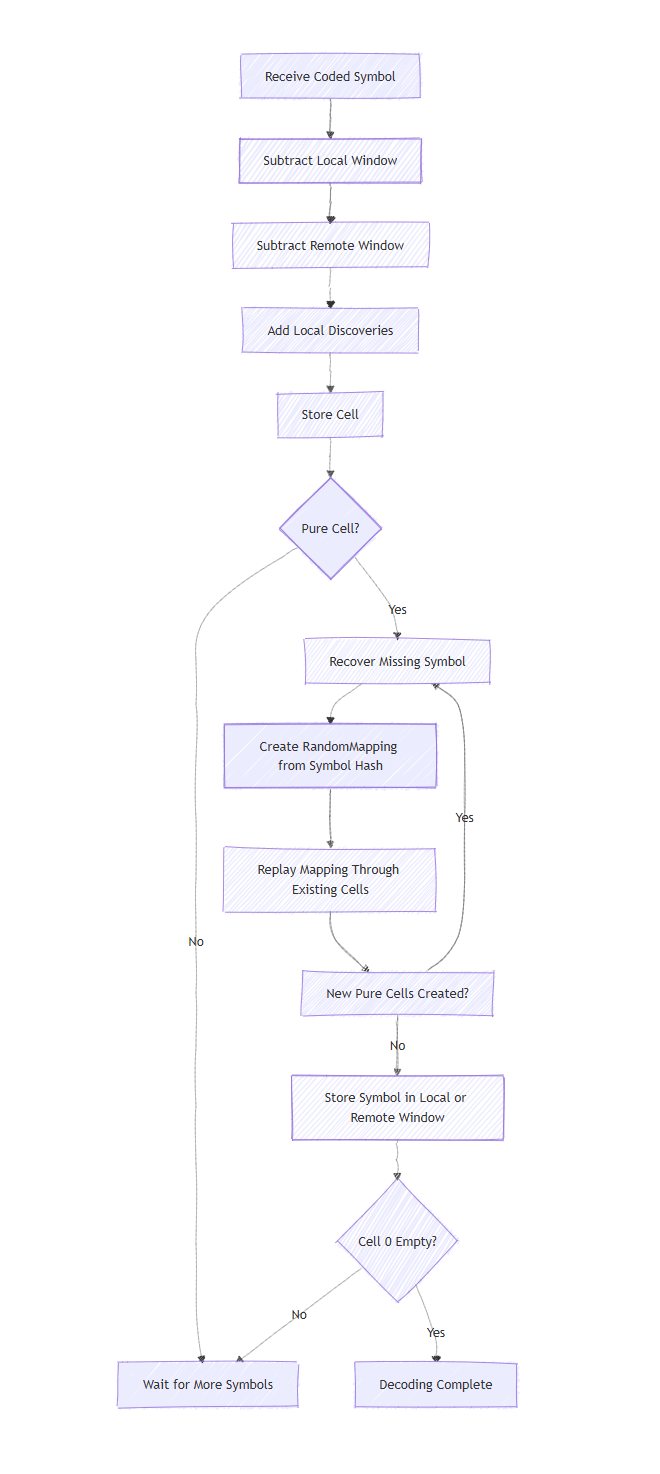
The job of the decoder is to process an incoming sequence of coded symbols and extract source symbols (cache mutations). Rather than ⊕'ing 2 static arrays like in the regular IBLT case, the decoder operates as a sort of continuous pipeline. Every received coded symbol undergoes a sequence of state-logical subtractions: the decoder removes the known LocalWindow and RemoteWindow, then adds back any LocalDiscoveries.
Once this known state is stripped away, the resulting cell is stored and evaluated to determine if it has become a pure cell. Recall from the IBLT section that a pure cell is one that contains exactly 1 unresolved mutation. We can verify this purity in O(1) time: if a cell's Count is exactly 1 or -1, and its CheckSum precisely matches the hash of its SymbolSum, the cell is pure (in other words "decodable").
When a pure cell is identified, the decoder extracts the missing symbol and triggers a peeling cascade. Because the PRNG mapping is deterministic, it creates a RandomMapping from the recovered symbol's hash and replays that mapping through the existing cells. It ⊕'s the mutation out of those other cells. As mutations are peeled away, previously entangled cells (k-cores) may suddenly become pure, triggering a loop of new discoveries (as seen in the "New Pure Cells Created?" feedback loop in flow diagram of the decoder).
Once the peeling cascade stops, the recovered symbols are stored in their respective windows (see definitions above). Finally, the decoder checks its termination condition: if cell 0 is completely empty, decoding is complete. Otherwise, it waits for more symbols to arrive from the rateless stream.
internal class RibltDecoder
{
    private readonly CodingWindow _current = new();
    private readonly CodingWindow _local = new();
    private readonly CodingWindow _remote = new();

    private readonly List<CodedSymbol> _cells = [];
    private readonly List<int> _decodableIndexes = [];

    public bool IsCompleted
    {
        [MethodImpl(MethodImplOptions.AggressiveInlining)]
        get => _cells.Count > 0 && _cells[0].IsEmpty;
    }

    public void TryDecode()
    {
        var span = CollectionsMarshal.AsSpan(_cells);

        for (int i = 0; i < _decodableIndexes.Count; i++)
        {
            int cellIndex = _decodableIndexes[i];
            ref var codedSymbol = ref span[cellIndex];

            switch (codedSymbol.Count)
            {
                case 0: // Count = 0 means its empty, so nothing to extract.
                    break;
                case 1:
                    {
                        // Count == 1 means the remote has this item, but I dont have it.
                        // Because the cell is pure, the SymbolSum IS the actual MutationSymbol.Id
                        // We extract it by XOR'ing it with an empty default struct.

                        var hashedSymbol = new HashedSymbol(default(MutationSymbol).Xor(codedSymbol.SymbolSum), codedSymbol.CheckSum);

                        var mapping = ApplyNewSymbol(hashedSymbol, SymbolOperation.Remove, span);

                        _remote.AddHashedSymbol(hashedSymbol, mapping);

                        break;
                    }
                case -1:
                    {
                        // Count == -1 means this is an item I have, but the remote node is missing.
                        // Again the cell is pure, and we apply the same XOR'ing but this time we add this item
                        // back into the previpusly recevied cells, and save it so we can apply it to future cells.

                        var hashedSymbol = new HashedSymbol(default(MutationSymbol).Xor(codedSymbol.SymbolSum), codedSymbol.CheckSum);
                        var mapping = ApplyNewSymbol(hashedSymbol, SymbolOperation.Add, span);

                        _local.AddHashedSymbol(hashedSymbol, mapping);

                        break;
                    }
                default:
                    throw new UnreachableException($"Cell was marked as decodable, but Count is = {codedSymbol.Count}");
            }
        }

        _decodableIndexes.Clear();
    }

    private RandomMapping ApplyNewSymbol(HashedSymbol hashedSymbol, SymbolOperation operation, Span<CodedSymbol> cells)
    {
        var mapping = new RandomMapping(hashedSymbol.Hash, 0);

        // We only care about applying this to cells we have received so far.
        while (mapping.LastIndex < cells.Length)
        {
            int cellIndex = (int)mapping.LastIndex;

            cells[cellIndex].Apply(hashedSymbol, operation);

            if (cells[cellIndex].IsDecodable)
            {
                _decodableIndexes.Add(cellIndex);
            }

            mapping.NextIndex();
        }

        return mapping;
    }
}
When utilizing a sketch, the initial ⊕ between 2 nodes already neutralizes their shared state. To capitalize on this, the decoder exposes an optimized ingestion path via ApplyDifferenceSymbol().
// Used for when there is no sketch, or it has been out-grown!
public void ApplySymbol(CodedSymbol symbol)
{
    symbol = _current.ApplySymbol(symbol, SymbolOperation.Remove);
    symbol = _remote.ApplySymbol(symbol, SymbolOperation.Remove);
    symbol = _local.ApplySymbol(symbol, SymbolOperation.Add);

    _cells.Add(symbol);

    if (symbol.IsDecodable || symbol.IsEmpty)
    {
        _decodableIndexes.Add(_cells.Count - 1);
    }
}

// Used for when there is a sketch, and it has not been out-grown!
// Bypasses the baseline subtraction phase, as the caller has already
// neutralized overlapping state.
public void ApplyDifferenceSymbol(CodedSymbol diffSymbol)
{
    diffSymbol = _remote.ApplySymbol(diffSymbol, SymbolOperation.Remove);
    diffSymbol = _local.ApplySymbol(diffSymbol, SymbolOperation.Add);

    _cells.Add(diffSymbol);

    if (diffSymbol.IsDecodable || diffSymbol.IsEmpty)
    {
        _decodableIndexes.Add(_cells.Count - 1);
    }
}
Instead of performing an O(N) subtraction against the entire local window (the local cache's baseline) for every incoming symbol, this method accepts the pre-⊕'d difference directly. It only applies the small subset of mutations that have already been resolved during ongoing cascade iterations, thereby removing newly identified remote items, and adding local discoveries to keep the mathematical state current.
Once adjusted, the symbol is appended to the internal cells list. If this targeted subtraction successfully isolates a single mutation (making the cell pure), its index is immediately queued to feed the next phase of the peeling loop.
The diagram below gives an overview of how the decoder handles the incoming sequence of coded symbols, and extraction of source symbols.
Replication Engine
With the mathematical foundations set, we can now built a cache replication engine which achieves zero-hop local reads, while guaranteeing eventual consistency across the cluster. We lean heavily onto Orleans for providing robust cluster membership, and the ability to facilitate peer-to-peer communication.
To understand how this replication works we look at it through 2 lenses:
- The macro-level cluster topology that drives the cache replication.
- The micro-level node mechanics that operates on the cache items.
The following diagram gives a good overview of the macro-level lense.
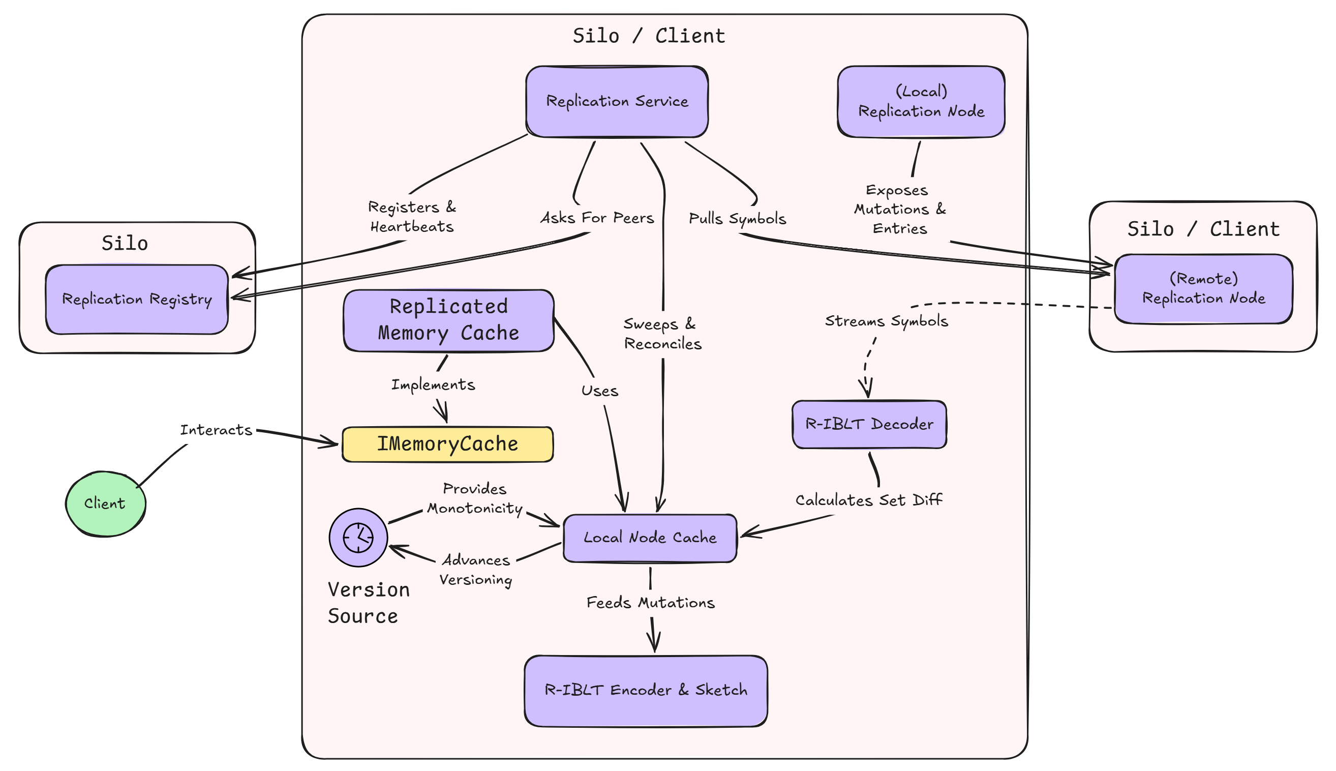
At its highest level, the engine is a decentralized mesh of silos and clients operating without a central replication coordinator. We refer to both silos and clients as "nodes". The anchor of this topology is the ReplicationRegistry. This remote registry acts as a node directory, where every active participant registers itself and emits periodic heartbeats to prove its health and availability. The registry employs direct & in-direct probing to ensure the nodes are healthy.
Eventhough the registry is a central point in regards to finding and maintaining a list of nodes, it does not participate on the actual movement of the data, that is handled in a decentralized way by the respective ReplicationService(s), which are local to every single node. Rather than broadcasting state to the entire cluster, this service employs a gossip protocol. It periodically asks the registery to pick a random peer node (which can be a silo or client) to initiate a reconciliation round with.
When the registry has picked a node, the local service reaches across the network to interact with that peer's ReplicationNode (which is remote to the service). However, nodes do not exchange raw cache payloads. Instead, the remote node exposes its local state as a stream of R-IBLT coded symbols. As elaborated above, the coded symbols are the mathematical mapping of the source symbols, which in our case are the IDs of the mutations done to each cache item. This stream is pulled continuously over the wire and piped into the R-IBLT decoder of the initiating node. The decoder than continuously peels away pure cells to calculate the exact set difference between the 2 nodes.
Once the decoder finds the exact set difference, the node (Node A) explicitly requests only the specific missing cache mutations from its peer (Node B). Because the set difference allows bi-directional identification of missing symbols, Node A is also able to tell Node B that it is missing cache items that Node A has in addition to Node A finding out that it is missing items present in Node B.
In this design, a cache mutation is the fundamental unit of state change. Rather than treating a cache entry as a mutable key-value pair, every modification is packaged into a self-contained versioned payload.
This mutation (precisely its ID) acts as the raw source symbol that gets encoded and decoded by the R-IBLT algorithm. These mutations flow directly into the LocalNodeCache (which the implementation of the standard IMemoryCache interface uses within it), so that consuming client applications interact with local memory at native speeds, remaining unaware of the ongoing background reconciliations.
At this level, maintaining thread concurrency is necessary. Locking the entire cache dictionary during reconciliation would reduce client operations throughput significantly, and swapping in a Dictionary under a single lock (while technically correct) would just drag on the Get() hot-path and the gossip thread's journal walk behind every writer.
Instead concurrency is layered: ConcurrentDictionary keeps each key structurally intact for its lock-free readers, while lock-striping guards what no single collection can which is cross-collection correctness such as: version check, cache/journal pairing, sketch updates, that all must happen atomically.
internal class LocalNodeCache
{
    private sealed record CacheEntry(byte[]? Payload, VersionTag Version,
        bool IsTombstone, DateTimeOffset? ExpiresAt, Guid MutationId);

    private readonly LocalNodeClock _source = new(Guid.NewGuid().GetHashCode());
    private readonly ConcurrentDictionary<string, CacheEntry> _cache = new();
    private readonly ConcurrentDictionary<Guid, CacheMutation> _mutations = new();

    private const int LockCount = 1024; // MUST be a power of 2 for bitwise masking.
    private const int LockMask = LockCount - 1;

    private readonly Lock[] _lockStrip = [.. Enumerable.Range(0, LockCount).Select(_ => new Lock())];

    public IEnumerable<CacheMutation> Mutations => _mutations.Values;

    public RibltSketch? Sketch { get; private set; } = options.MaterializedSketchSize > 0 ? new(options.MaterializedSketchSize) : null;

    public CacheMutation? GetMutation(Guid id) => _mutations.TryGetValue(id, out var mutation) ? mutation : null;

    /// <summary>
    /// Applies <paramref name="action"/> to all mutations local to this node.
    /// </summary>
    public void ForEachMutation<TState>(TState state, Action<TState, MutationSymbol> action)
    {
        // Instead of the encoder/decoder using the keys of the dict (which are the mutation ids),
        // we iterate over the dict directly to avoid boxing the Guid keys, and apply the action to each.
        // This is more efficient for large dictionaries, and I expect the number of mutations to be large in a busy cache.

        foreach (var kvp in _mutations)
        {
            action.Invoke(state, new MutationSymbol(kvp.Key));
        }
    }

    [MethodImpl(MethodImplOptions.AggressiveInlining)]
    private Lock GetLock(string key) => _lockStrip[(uint)key.GetHashCode() & LockMask];

    public byte[]? Get(string key)
    {
        if (_cache.TryGetValue(key, out var entry) && !entry.IsTombstone)
        {
            if (entry.ExpiresAt.HasValue && entry.ExpiresAt.Value <= timeProvider.GetUtcNow())
            {
                // This is a logical eviction, meaning the entry is here but its time is up!
                // We dont need to remove the entry as the period sweep will take care of it.

                return null;
            }

            return entry.Payload;
        }

        return null;
    }

    public void Set(string key, byte[] value, TimeSpan? ttl = null)
    {
        var utcNow = timeProvider.GetUtcNow();

        ApplyMutation(new CacheMutation
        {
            MutationId = Guid.NewGuid(),
            Version = _source.GetNextVersion(utcNow.Ticks),
            CacheKey = key,
            IsTombstone = false,
            PayloadBytes = value,
            PayloadHash = value.Length > 0 ? StableHash.ComputeHash(value) : 0,
            ExpiresAt = ttl.HasValue ? utcNow + ttl.Value : null
        });
    }

    public void Remove(string key) => ApplyMutation(new CacheMutation
    {
        MutationId = Guid.NewGuid(),
        Version = _source.GetNextVersion(timeProvider.GetUtcNow().Ticks),
        CacheKey = key,
        IsTombstone = true,
        PayloadBytes = null,
        PayloadHash = 0,
        ExpiresAt = null
    });

    public void ApplyMutation(CacheMutation mutation)
    {
        if (mutation.ExpiresAt.HasValue &&
            timeProvider.GetUtcNow() > mutation.ExpiresAt.Value + _mutationGracePeriod)
        {
            // It can be that lagging node applies the
            // mutation but it is already objectively expired.
            // Like, the sweeping has already occurred in
            // this (receiver) node, so we wont re-add it!
            return;
        }

        // If this mutation came from a node whose clock is ahead of ours,
        // we artificially advance our clock to match it.
        _source.CatchUp(mutation.Version.Ticks);

        var cacheKey = mutation.CacheKey;

        lock (GetLock(cacheKey))
        {
            if (_cache.TryGetValue(cacheKey, out var existing))
            {
                if (mutation.Version <= existing.Version)
                {
                    // If the incoming mutation is older or a duplicate,
                    // its safe to discard it.
                    return;
                }

                // To prevent a memory leak, we are overwriting the key,
                // so we MUST remove the old mutation id from the journal.
                _mutations.TryRemove(existing.MutationId, out _);

                // We also remove the old mutation from the sketch,
                // so that it is not sent to other nodes anymore.
                Sketch?.ApplyMutation(new MutationSymbol(existing.MutationId), SymbolOperation.Remove);
            }

            // Then we atomically update both collections!
            _mutations[mutation.MutationId] = mutation;
            _cache[cacheKey] = new CacheEntry(mutation.PayloadBytes, mutation.Version, mutation.IsTombstone, mutation.ExpiresAt, mutation.MutationId);

            // We also add the new mutation to the sketch,
            // so that it is sent to other nodes.
            Sketch?.ApplyMutation(new MutationSymbol(mutation.MutationId), SymbolOperation.Add);
        }
    }

    public void SweepExpiredMutations()
    {
        var utcNow = timeProvider.GetUtcNow();

        // We only need to iterate over _cache because every valid mutation is tracked there.
        foreach (var kvp in _cache)
        {
            var key = kvp.Key;

            lock (GetLock(key))
            {
                // Need to double-check the state inside the lock to ensure it hasnt been updated
                // by a user shortly before the sweep got triggered.

                if (_cache.TryGetValue(key, out var entry) && entry.ExpiresAt.HasValue)
                {
                    if (utcNow > entry.ExpiresAt.Value + _mutationGracePeriod)
                    {
                        // We can safely remove both, without risking a race conditions with ongoing reads/writes.
                        _cache.TryRemove(key, out _);
                        _mutations.TryRemove(entry.MutationId, out _);
                        // We also remove the old mutation from the sketch, so that it is not sent to other nodes anymore.
                        Sketch?.ApplyMutation(new MutationSymbol(entry.MutationId), SymbolOperation.Remove);
                    }
                }
            }
        }
    }
}
By mapping cache keys to an array of dedicated locks, background reconciliation streams can write missing mutations in parallel without blocking local client operations on unrelated keys, and ForEachMutation() samples the journal in a weakly consistently fashion, so encoding never stalls a writer.
It is understanable to worry that 2 threads applying mutations to different cache keys (each holding a different stripe lock) could still corrupt shared state. They can not though, because the sketch employs its own internal lock-striping as we discussed above. And since locks are only ever acquired in one direction: cache stripe → cell stripe, the 2 components can work together without introducing a deadlock risk (to my best knowledge).
Monotonicity & Versioning
To handle concurrent modifications deterministically without relying on global locks, each node maintains a custom, strictly monotonic source of versioning. A physical wall clock alone can not guarantee monotonically increasing timestamps as the local clock may move backward due to NTP adjustments, clock drift, or what not. While a purely logical clock provides ordering information but has no direct relationship to physical elapsed time, and therefore can not by itself be used to evaluate TTL-based cache expirations.
VersionSource combines the 2 properties without explicitly maintaining separate physical and logical components. For each locally generated version, the next value is computed as the maximum of the current physical timestamp, and the previous version (incremented by 1):
next = max(physicalTicks, currentVersion + 1);Consequently, when physical time has advanced beyond the previous version, the generated version follows physical time. If physical time has not advanced sufficiently (or has moved backwards) the logical increment takes precedence, ensuring that every locally generated version is strictly monotonic.
internal class VersionSource(int nodeId)
{
    private long _version;

    [MethodImpl(MethodImplOptions.AggressiveInlining)]
    public VersionTag GetNextVersion(long physicalTicks)
    {
        long current;
        long next;

        do
        {
            current = Interlocked.Read(ref _version);

            // The new time must be strictly *greater* than the previous time.
            // If physical time is behind due to clock drift, we force it forward by (+1).

            next = Math.Max(physicalTicks, current + 1);
        }
        // So long as the current version is not equal to the value we read, we will retry the update.
        // This is because another thread may have updated the version in between our read and write.
        while (Interlocked.CompareExchange(ref _version, next, current) != current);

        return new VersionTag(next, nodeId);
    }

    [MethodImpl(MethodImplOptions.AggressiveInlining)]
    public void CatchUp(long incomingTicks)
    {
        long current;

        // If an incoming gossip mutation is from the "future", we advance our version!
        while (incomingTicks > (current = Interlocked.Read(ref _version)))
        {
            // CompareExchange returns the original value, so we loop until we successfully update the version,
            // in case of concurrent updates from other threads.
            Interlocked.CompareExchange(ref _version, incomingTicks, current);
        }
    }
}
The version (value) is stored as a single 64-bit long, allowing the update to be performed atomically using Interlocked operations. This makes concurrent version generation lock-free (as every mutation has to go through this): if another thread modifies the version between the initial read and the CAS loop, the operation fails and is retried using the newly observed value.
VersionSource is also advanced when a mutation is received from another node. If the incoming mutation carries a version greater than the local version, CatchUp advances the local version to that value. Consequently, any subsequently generated local version will be greater than a version that the node has already observed. This allows for causal ordering across replicated mutations, without requiring the physical clocks of different nodes to be perfectly synchronized.
A version is represented by a VersionTag, which contains both the generated tick value, and the ID of the node that generated it.
internal readonly record struct VersionTag(long Ticks, int NodeId)
    : IComparable<VersionTag>
{
    public int CompareTo(VersionTag other)
    {
        var cmp = Ticks.CompareTo(other.Ticks);
        return cmp != 0 ? cmp : NodeId.CompareTo(other.NodeId);
    }
}
Versions are compared lexicographically, so the tick value is compared first, and the node ID is used as a deterministic tie-breaker when 2 versions have identical ticks. This gives the system a total ordering over mutations. A mutation with a greater VersionTag is considered newer, while an older or identical version can be discarded.
When a mutation is about to be applied, the receiver node (precisely the local cache of that node) first "catches up" its local VersionSource, and then compares the incoming version against the version currently associated with the cache key. If the incoming version is not greater the mutation is ignored, otherwise it replaces the existing mutation and its associated journal and cache entries.
Version ordering and expiration are kept conceptually separate. VersionTag determines which mutation wins, whereas ExpiresAt is evaluated using the physical time. This prevents the logical version mechanism from being incorrectly treated as a measurement of elapsed time. A mutation can therefore lose a version comparison because a newer mutation exists, while expiration independently determines whether an otherwise valid mutation should still be obserable on a receiving node.
Together, the VersionSource and VersionTag provide deterministic conflict resolution without requiring globally synchronized clocks: the version source guarantees strict monotonicity on each node (and accounts for observed remote versions), while NodeId guarantees deterministic ordering when independent nodes produce identical tick values.
Finally, to complete the cycle and prepare for future gossips, every local mutation is immediately written into the encoder & sketch. While the sketch is optional, it is recommended to have one alongside the local state, as the node can absorb state updates without triggering the cell-0 avalanche effect i.e. the cold-start. The ReplicationService uses the sketch as a fast-path optimization for the decoder, while the ReplicationNode uses it for the encoder.
The interesting part here is how the sketch and the encoder work together. The sketch is essentially the cheap, already-materialized version of the beginning of the symbol stream, while the encoder is used as a fallback when the sketch is exhausted or disabled.
When the remote ReplicationNode receives a request for symbols, it first checks whether it has a sketch and whether the requested offset falls within its capacity. If so, it simply reads the required slice from the sketch and returns it. This is the fast path i.e. the symbols have already been materialized, so there is no need to construct or advance an encoder just to serve them.
if (localCache.Sketch is { } sketch && state.Offset < sketch.Size)
{
    var countToRead = Math.Min(batchSize, sketch.Size - state.Offset);

    CollectionsMarshal.SetCount(symbols, countToRead);

    var destSpan = CollectionsMarshal.AsSpan(symbols);
    var readCount = sketch.ReadSlice(state.Offset, destSpan);

    state.Offset += readCount;
    batchSize -= readCount;
}
On the other side, the ReplicationService does not care where these symbols came from. It requests batches from the remote node and feeds whatever it receives directly into its decoder. This keeps the protocol nice and simple because from the service's perspective the remote node is just exposing a stream of coded symbols.
Once the sketch has been exhausted, the remote node needs to continue the same symbol stream using an encoder. If one has not already been created, it creates and starts hydrating one in the background rather than doing all of that work synchronously inside the grain.
if (state.Encoder is null)
{
    if (state.HydrationTask is null)
    {
        state.HydrationTask = Task.Run(() =>
        {
            var encoder = new RibltEncoder();

            // We start the encoder from the target offset,
            // which may be beyond the sketch size,
            // to ensure we produce the correct symbols.
            // Essentially we fast-forward the encoder to the desired offset,
            // skipping over any symbols that have already been created
            // (and served on a previous batch round) in the sketch.

            localCache.ForEachMutation((encoder, targetOffset), (state, mutation) =>
                state.encoder.AddMutationAtOffset(mutation, state.targetOffset));

            return encoder;
        });
    }

    if (!state.HydrationTask.IsCompleted)
    {
        return symbols.AsImmutable();
    }

    state.Encoder = await state.HydrationTask;
    state.HydrationTask = null;
}
There is an important detail here: the encoder is fast-forwarded to the current stream offset. This means that if the sketch already served, say the first 1,000 symbols, the encoder does not start again from the 0th symbol. It is advanced to symbol 1,000 and continues from there. From the peer's perspective, it is still receiving one continuous symbol stream, it does not need to know that the first part came from a sketch, and the rest came from an encoder.
Hydrating the encoder can be quite expensive for large caches, so this work is deliberately offloaded to the Thread Pool. While the hydration task is still running, the remote node returns an empty batch instead of blocking the grain. The initiating service can then back off and retry the request shortly afterwards. Once the encoder is ready, symbol generation continues normally.
const int MaxTimeSliceMs = 2;

var startTime = Stopwatch.GetTimestamp();

for (int i = 0; i < batchSize; i++)
{
    var symbol = state.Encoder.ProduceNextSymbol();

    symbols.Add(symbol);
    state.Offset++;

    if ((i & 255) == 0 && Stopwatch.GetElapsedTime(startTime).TotalMilliseconds >= MaxTimeSliceMs)
    {
        await Task.Yield();
        startTime = Stopwatch.GetTimestamp();
    }
}
Generating coded symbols can become CPU-intensive on large caches, so the encoder also has a small CPU-yielding safeguard. We periodically yield during symbol generation to prevent a large batch from monopolizing the grain thread. The elapsed time is checked every 256 iterations, and once at least ~2 [ms] have passed, we yield to the scheduler. This creates a nice sweet spot where:
- We yield at ~2 [ms] of actual CPU time per execution slice.
- We dilute the overhead of calling the stopwatch and yielding.
- We maximize throughput while preventing grain thread starvation.
This way the ReplicationNode can serve symbols to another node (in a turn-based fashion), but also is readily available for probing by the registry (or indirectly from another node). The 2 [ms] is somewhat empirical in that it is roughly sufficient to cover the base symbol stream batch size (default of 256) for a small-ish caches. Therefore we use it as a baseline for larger caches, where generating the same batch may take longer and the loop can cooperatively yield as needed. The value is also well within Orleans' activation scheduling quantum, keeping the work "digestible" for the grains turn-based execution.
The sequence diagram below gives an overview of how the replication engine operates between 2 peers.
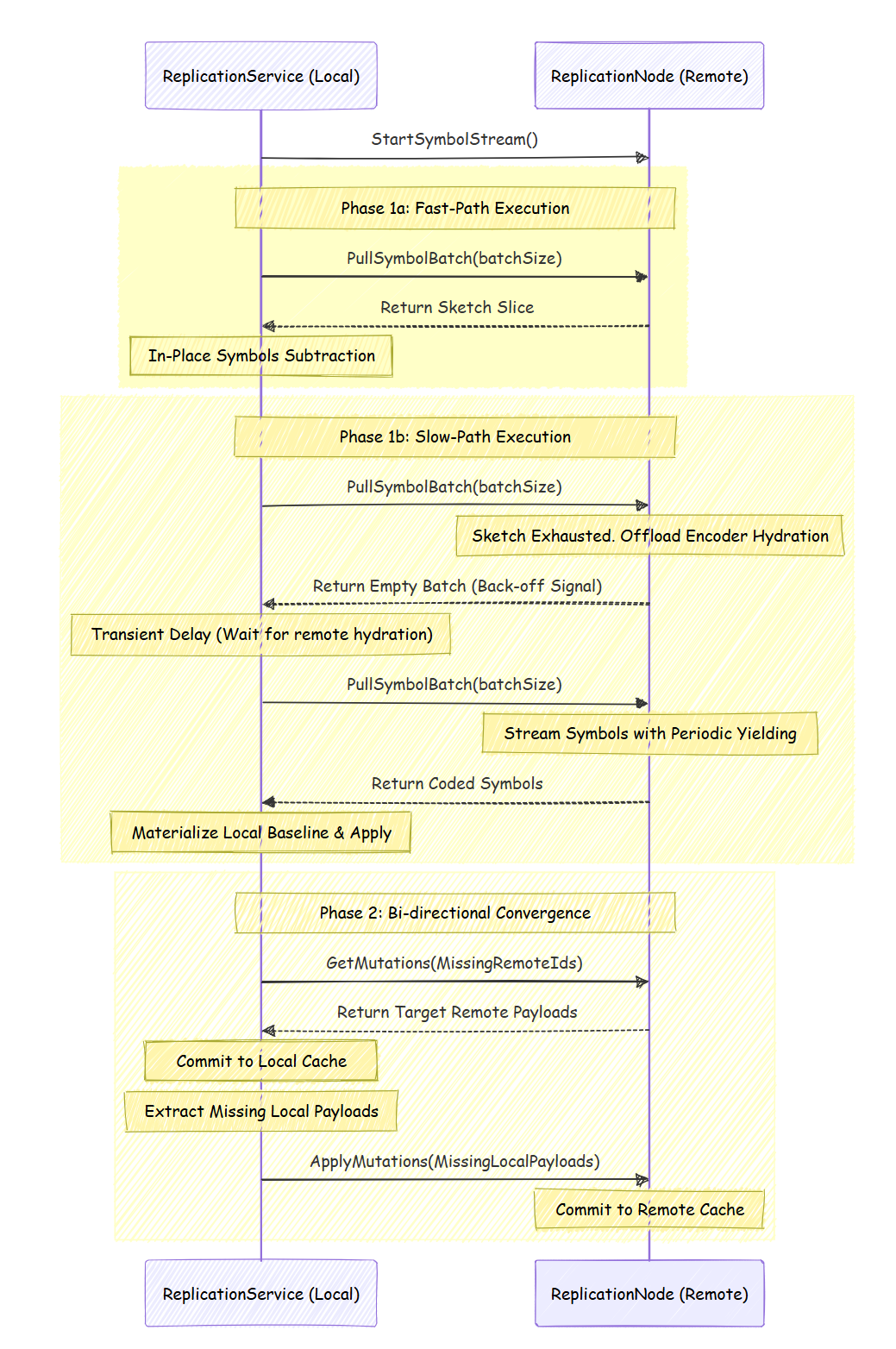
Stress Testing
In order to test how the engine holds up under concurrent traffic, we spin up a 3-node Orleans cluster and hit it with a sustained load generator. The test setup uses 25 worker threads aiming for 10,000 [ops/s] across the cluster. While the workers mutate and read the cache, a dedicated background thread quite aggressively samples random keys across all nodes simultaneously, and calculates the real-time convergence rate (how often all nodes agree on the value of any given key of a cache entry).
We run the load for exactly 10 [s] which is the stress phase in the convergence timeline diagram, then halt the traffic and move into a cooldown phase to measure how fast the cluster heals itself. The test matrix iterates through multiple configurations, repeating each setup 3 times to average out the results.
| Parameter | Configurations |
|---|---|
| Worker Threads | 25 |
| Target Load | 10,000 [ops/s] |
| Write/Read Ratio | 10%, 30%, 50% |
| Reconciliation Period | 50 [ms], 100 [ms], 500 [ms], 1000 [ms] |
Convergence Timelines
Looking at the diagram below, the red shaded area is the stress phase, while the green area is the cooldown phase.
When the systen is configured with a tight 50-100 [ms] reconciliation period, it fights back the entropy almost instantly. Despite the heavy write contention, these aggressive configurations find their way to near 100% convergence within the first 1.5-2 [sec], and maintain it throughout the stress phase.
Extending the period to 500-1000 [ms] forces the nodes to tolerate much higher state drift. During the stress phase, these slower configurations hover around a lower (though remarkably close) convergence floor. However, the moment the load generator shuts off at the 10 [s] mark, these configurations snap up to a full 100%.
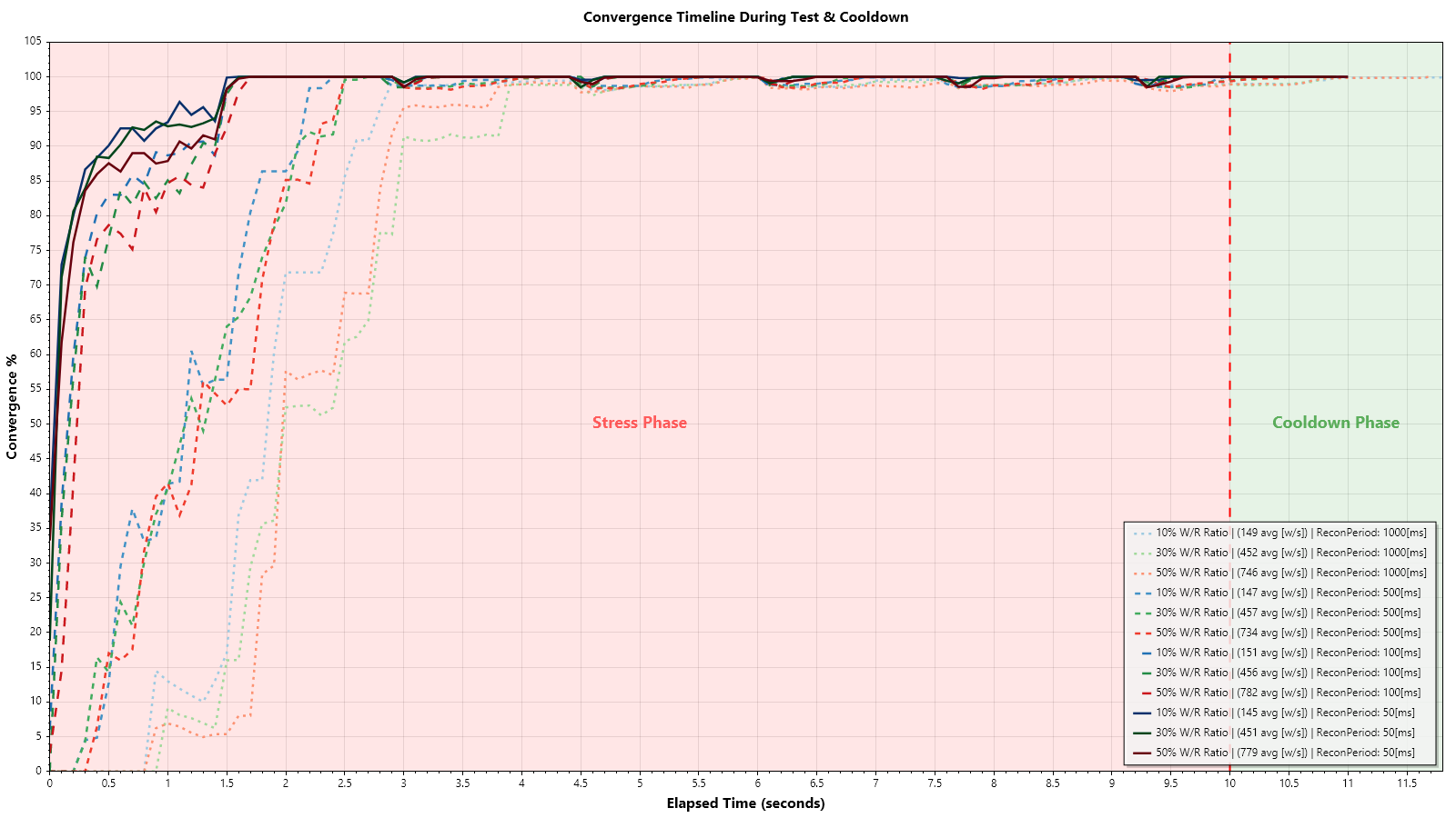
Consistency Floors
The median P50 is a nice vanity metric, but we want to be judged by the worst-case scenario. The diagram below breaks down the P50, P05, and P01 tail-end convergence percentiles during the stress phase to show the absolute floor of our data consistency.
At an aggressive 50 [ms] reconciliation period, with a 10% write ratio (averaging about 148 [writes/sec]), the system is virtually bulletproof. The median P50 sits perfectly at 100%, the P05 sits at a respectable 88%, and even the absolute worst case of the P01 the nodes agree on the cache entries 47% of the time.
Eventually everything has to crack of course! If we increase the write ratio up to 50% (pushing ~760 [writes/sec]) and increase the reconciliation period to 1000 [ms], the system sacrifices real-time consistency. The median stays remarkably high at 99%, but P05 and P01 plummet to 1%.
This visualizes the fundamental trade-off of the design. You can dial down the reconciliation period to maintain incredibly tight consistency floors (even under heavy write contention), at the cost of higher CPU utilization. Or, if you can tolerate stale reads, you can dial it up, thereby saving CPU cycles and bandwidth while trusting that the mathematical baseline will eventually (in reality this will be very fast when traffic slows down) force the cluster back into perfect sync.
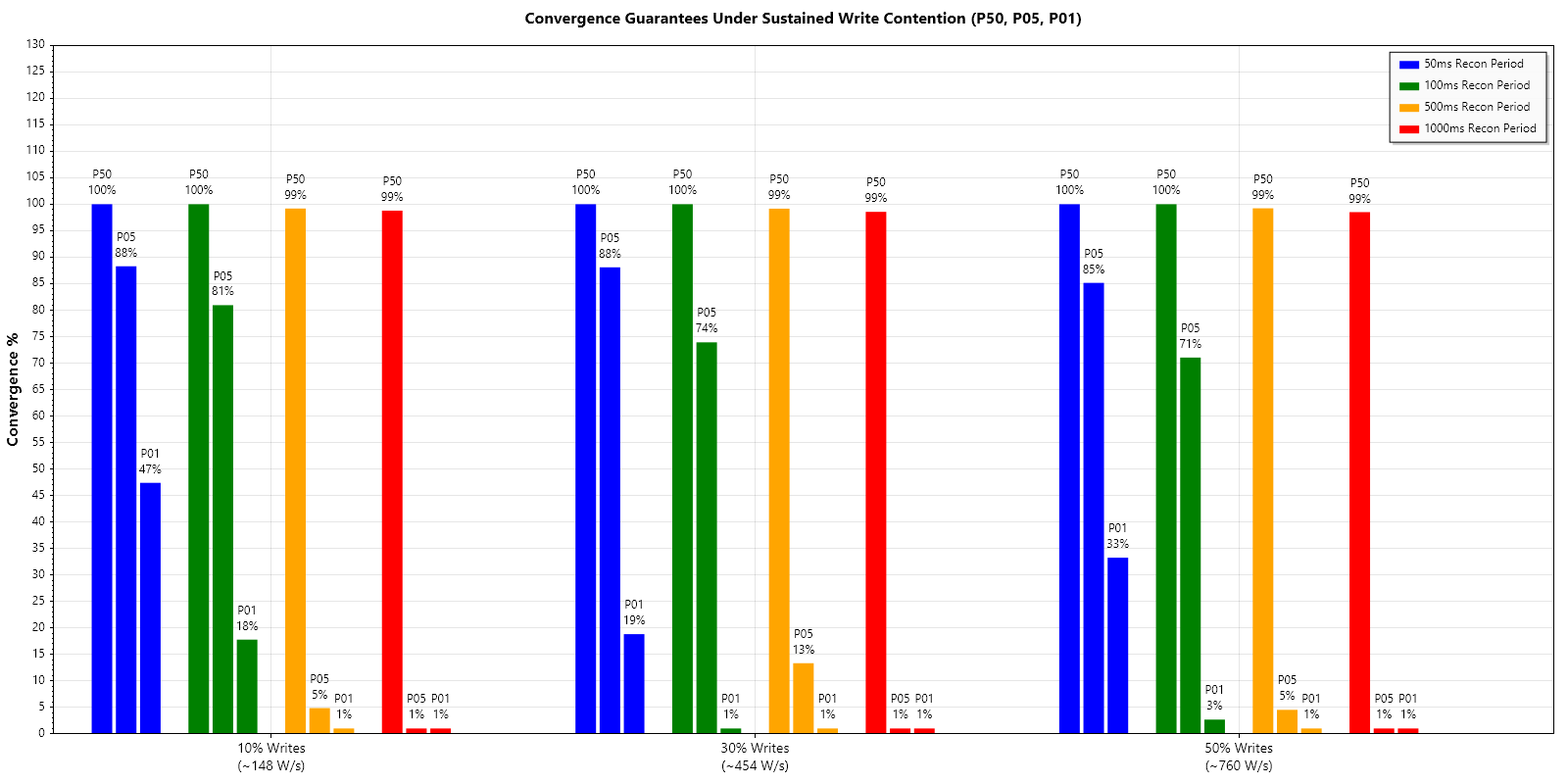
Expiration Semantics
In traditional in-process or centralized caches, sliding expiration extends an item's lifetime every time it is read. In a decentralized 0-hop replication setup, doing this across nodes would require communicating every local read to the other nodes, which would defeat the purpose of fast local reads.
To keep reads fully local, SlidingExpiration is treated as AbsoluteExpirationRelativeToNow when the cache entry is committed. In other words, the sliding expiration value becomes the item's initial TTL, rather than being extended on every read. This keeps cache reads strictly local and avoids network traffic or additional work on every GET. The trade-off is that a read does not extend the item's lifetime. The expiration can only change when the entry is explicitly updated or the state is reconciled again.
Entries with a zero or even negative TTLs are treated as explicit removals rather than normal cache entries. These removals are represented as tombstones so they can be propagated through the R-IBLT reconciliation process. Because these tombstones are kept long enough to be seen by other nodes during reconciliation, they eventually get cleaned up. This prevents old tombstones from unnecessarily increasing sketch size and negatively impacting the reconciliation performance.
private class CacheEntry(string key,
    TimeProvider timeProvider, LocalNodeCache localCache,
    ICacheEntrySerializer serializer) : ICacheEntry
    {
        ...

        public void Dispose()
        {
            ...

            TimeSpan? ttl = null;

            if (AbsoluteExpirationRelativeToNow.HasValue)
            {
                ttl = AbsoluteExpirationRelativeToNow.Value;
            }
            else if (AbsoluteExpiration.HasValue)
            {
                ttl = AbsoluteExpiration.Value - timeProvider.GetUtcNow();
            }
            else if (SlidingExpiration.HasValue)
            {
                ttl = SlidingExpiration.Value;
            }

            if (ttl.HasValue && ttl.Value <= TimeSpan.Zero)
            {
                localCache.Remove((string)Key);
                return;
            }

            localCache.Set((string)Key, serializer.Serialize(Value), ttl);
        }
    }
}
Why R-IBLTs?
In a highly dynamic distributed cluster, nodes spin up and down at non-regular intervals, and the exact volume of missed cache mutations between any 2 silos/clients can easily become unpredictable. R-IBLTs solve this challenge without compromising performance.
Standard IBLTs require you to guess the number of differences upfront (in order to size the data structure itself). R-IBLTs instead generate an infinite sequence of coded symbols. A receiving node process these symbols until it successfully reconciles its state, completely removing the need for size estimation.
Full-sync algorithms (where nodes exchange their entire dataset) scale with the total data size, rather than the size of the difference. This results in massive, unnecessary data transfers that may choke network bandwidth as the cluster state grows.
While alternatives like PinSketch achieve optimal communication bandwidth, their decoding phase is very CPU intensive. R-IBLTs scale linearly and operates up to 2000x faster than PinSketch for computation.
R-IBLTs operate near the theoretical communication minimum. Unlike Merkle Trees (or more precisely Patricia Tries), they can often resolve set differences in a single network hop, without requiring chattiness between peers.
For detailed information on the performance of R-IBLTs, please refer to the paper. Generally by utilizing R-IBLTs, the replication engine keeps network payloads small and very predictable, while placing minimal burden on the CPU.
If you found this article helpful please give it a share in your favorite forums 😉.
The solution project is available on GitHub.